Fitting multivariate ODE models with brms
This article illustrates how ordinary differential equations and multivariate
observations can be modelled and fitted with the brms package (Bürkner (2017)) in R1.
As an example I will use the well known Lotka-Volterra model (Lotka (1925), Volterra (1926)) that describes the predator-prey behaviour of lynxes and hares. Bob Carpenter published a detailed tutorial to implement and analyse this model in Stan and so did Richard McElreath in Statistical Rethinking 2nd Edition (McElreath (2020)).
Here I will use brms as an interface to Stan. With brms I can write the
model using formulas similar to glm or lmer directly in R,
avoiding to code up the model in Stan. Having said that, I will have to write
a little bit of Stan for the ODEs and pass them on via the brm
function.
Data
The data to model shows the number of pelts in thousands of Canadian hares and lynxes from 1900 - 1920:
library(data.table)
Lynx_Hare <- data.table(
  Year = 1900:1920,
  Lynx = c(4, 6.1, 9.8, 35.2, 59.4, 41.7, 19, 13, 8.3, 9.1, 7.4, 8,
           12.3, 19.5, 45.7, 51.1, 29.7, 15.8, 9.7, 10.1, 8.6),
  Hare = c(30, 47.2, 70.2, 77.4, 36.3, 20.6, 18.1, 21.4, 22, 25.4,
           27.1, 40.3, 57, 76.6, 52.3, 19.5, 11.2, 7.6, 14.6, 16.2, 24.7))
head(Lynx_Hare)
## Year Lynx Hare
## 1: 1900 4.0 30.0
## 2: 1901 6.1 47.2
## 3: 1902 9.8 70.2
## 4: 1903 35.2 77.4
## 5: 1904 59.4 36.3
## 6: 1905 41.7 20.6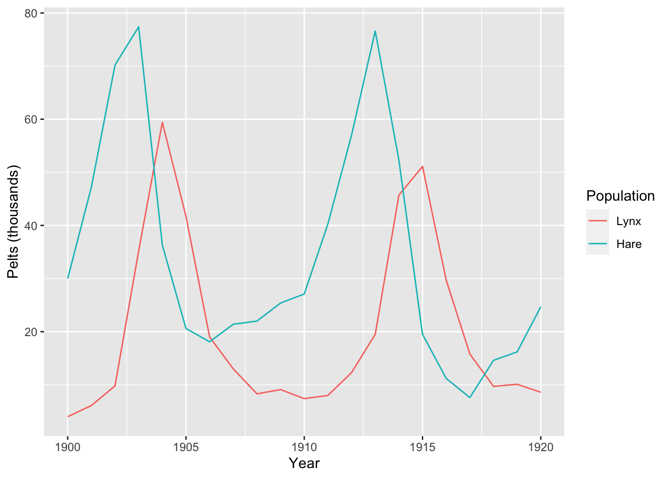
Model
The classic Lotka-Volterra model is a system of two autonomous ordinary differential equations (ODEs), describing the interaction between hares and lynxes. The four ODE parameters related to the birth and mortality rates of the two populations. In addition, there are two parameters for the initial states at time \(t=0\):
\[\begin{aligned} \frac{dH}{dt} & = (b_H - m_H L ) H \\ \frac{dL}{dt} & = (b_L H - m_L) L \\ H(0) & = H_0 \\ L(0) & = L_0 \\ \end{aligned}\]Note, the data only show the number of pelts, i.e. the number of trapped and killed animals not the actual population statistics.
Assuming no population can become extinct and all parameters have to be positive, I will assume log-normal distributions for the process and the birth and mortality parameters.
Implementation in brms
Load the R packages needed:
library(brms)
library(cmdstanr)
library(parallel)
nCores <- detectCores()
options(mc.cores = nCores)
Data preperations
The data was presented as a table with two columns, showing the time series for the hares and lynxes separately - a multivariate time series.
However, in order to model this data with brms the data has to be transformed
into a univariate time series. The trick is to introduce a dummy
variable for the long format of the data. In addition I add a new time variable,
which starts at 1, rather than 1900.
LH <- melt(data.table(Lynx_Hare), id.vars = "Year",
           measure.vars = c("Lynx", "Hare"),
           variable.name = "Population",
           value.name = "Pelts")
LH[, `:=` (
  delta = ifelse(Population %in% "Lynx", 1, 0),
  Population = factor(Population),
  t = Year - min(Year) + 1)]
head(LH)
## Year Population Pelts delta t
## 1: 1900 Lynx 4.0 1 1
## 2: 1901 Lynx 6.1 1 2
## 3: 1902 Lynx 9.8 1 3
## 4: 1903 Lynx 35.2 1 4
## 5: 1904 Lynx 59.4 1 5
## 6: 1905 Lynx 41.7 1 6ODE model in Stan
The implementation of the ODEs in Stan is straightforward, but note
below the integration step and the use of the dummy variable delta
from my data set and how I use it to select the relevant metric from the
bivariate output of the integrated ODEs. For delta = 0 the LV function
returns the hare component only and for delta = 1 the lynx component.
LotkaVolterra <- "
// Sepcify dynamical system (ODEs)
vector ode_LV(real t, vector y,  vector theta){
  vector[2] dydt;

  dydt[1] = (theta[1] - theta[2] * y[2] ) * y[1]; // Hare
  dydt[2] = (theta[3] * y[1] - theta[4]) * y[2]; // Lynx

  return dydt;
}
// Integrate ODEs and prepare output
real LV(real t, real Hare0, real Lynx0,
        real brHare, real mrHare,
        real brLynx, real mrLynx,
        real delta){
  vector[2] y0;     // Initial values
  vector[4] theta;  // Parameters
  array[1] vector[2]  y;   // ODE solution
  // Set initial values
  y0[1] = Hare0; y0[2] = Lynx0;
  // Set parameters
  theta[1] = brHare; theta[2] = mrHare;
  theta[3] = brLynx; theta[4] = mrLynx;
  // Solve ODEs
  y = ode_rk45(ode_LV, y0, 0, rep_array(t, 1), theta);
  // Return relevant population values
  return (y[1,1] * (1 - delta) + y[1,2] * delta);
}
"
Formula
To write the model formula in brms I make use of the nlf function,
short for non-linear function, not only to map the median behaviour of the
process, but also to transform standardised Normal(0, 1) priors to log-normal
priors. In addition, I allow for different process variances for the two
populations.
frml <-  bf(
  Pelts ~ eta,
  nlf(eta ~ log(
    LV(t, Hare0, Lynx0,
       brHare, mrHare,brLynx, mrLynx, delta)
    )
  ),
  nlf(Hare0 ~ 10 * exp(stdNHare0)),
  nlf(Lynx0 ~ 10 * exp(stdNLynx0)),
  nlf(brHare ~ 0.5 * exp(0.25 * stdNbrHare)),
  nlf(mrHare ~ 0.025 * exp(0.25 * stdNmrHare)),
  nlf(brLynx ~ 0.025 * exp(0.25 * stdNbrLynx)),
  nlf(mrLynx ~ 0.8 * exp(0.25 * stdNmrLynx)),
  stdNHare0 ~ 1,  stdNLynx0 ~ 1,
  stdNbrHare ~ 1, stdNmrHare ~ 1,
  stdNbrLynx ~ 1, stdNmrLynx ~ 1,
  sigma ~ 0 + Population,
  nl = TRUE)
Priors
Where possible I try to stick to standardised Normal priors and use nlf to
transform those to what I think are sensible ranges for the model.
mypriors <- c(
  prior(normal(0, 1), nlpar = "stdNHare0"),
  prior(normal(0, 1), nlpar = "stdNLynx0"),
  prior(normal(0, 1), nlpar = "stdNbrHare"),
  prior(normal(0, 1), nlpar = "stdNmrHare"),
  prior(normal(0, 1), nlpar = "stdNbrLynx"),
  prior(normal(0, 1), nlpar = "stdNmrLynx"),
  prior(normal(-1, 0.5), class = "b",
        coef= "PopulationHare",  dpar = "sigma"),
  prior(normal(-1, 0.5), class = "b",
        coef= "PopulationLynx",  dpar = "sigma")
  )
Model run
With the preparations done, I can start running the model with brm.
I use cmdstan as the backend and feed the ODE model using the stanvars
argument.
mod <- brm(
  frml, prior = mypriors,
  stanvars = stanvar(scode = LotkaVolterra, block = "functions"),
  data = LH, backend = "cmdstan",
  family = brmsfamily("lognormal", link_sigma = "log"),
  control = list(adapt_delta = 0.99),
  seed = 1234, iter = 1000,
  chains = 4, cores = nCores,
  file = "LotkaVolterraCMDStan.rds")
Model output
The model run takes about 3 minutes on my 2020 M1 MacBook Air. The output looks promising:
mod## Family: lognormal
## Links: mu = identity; sigma = log
## Formula: Pelts ~ eta
## eta ~ log(LV(t, Hare0, Lynx0, brHare, mrHare, brLynx, mrLynx, delta))
## Hare0 ~ 10 * exp(stdNHare0)
## Lynx0 ~ 10 * exp(stdNLynx0)
## brHare ~ 0.5 * exp(0.25 * stdNbrHare)
## mrHare ~ 0.025 * exp(0.25 * stdNmrHare)
## brLynx ~ 0.025 * exp(0.25 * stdNbrLynx)
## mrLynx ~ 0.8 * exp(0.25 * stdNmrLynx)
## stdNHare0 ~ 1
## stdNLynx0 ~ 1
## stdNbrHare ~ 1
## stdNmrHare ~ 1
## stdNbrLynx ~ 1
## stdNmrLynx ~ 1
## sigma ~ 0 + Population
## Data: LH (Number of observations: 42)
## Draws: 4 chains, each with iter = 1000; warmup = 500; thin = 1;
## total post-warmup draws = 2000
##
## Population-Level Effects:
## Estimate Est.Error l-95% CI u-95% CI Rhat Bulk_ESS
## stdNHare0_Intercept 0.87 0.09 0.70 1.04 1.00 1294
## stdNLynx0_Intercept -0.42 0.10 -0.62 -0.23 1.00 1103
## stdNbrHare_Intercept 0.20 0.35 -0.52 0.84 1.00 583
## stdNmrHare_Intercept 0.18 0.46 -0.75 1.06 1.00 671
## stdNbrLynx_Intercept -0.07 0.44 -0.93 0.83 1.00 653
## stdNmrLynx_Intercept 0.09 0.33 -0.54 0.76 1.00 574
## sigma_PopulationLynx -1.36 0.16 -1.66 -1.02 1.00 1585
## sigma_PopulationHare -1.39 0.17 -1.70 -1.05 1.01 1202
## Tail_ESS
## stdNHare0_Intercept 1243
## stdNLynx0_Intercept 1199
## stdNbrHare_Intercept 833
## stdNmrHare_Intercept 961
## stdNbrLynx_Intercept 802
## stdNmrLynx_Intercept 742
## sigma_PopulationLynx 1307
## sigma_PopulationHare 1026
##
## Draws were sampled using sample(hmc). For each parameter, Bulk_ESS
## and Tail_ESS are effective sample size measures, and Rhat is the potential
## scale reduction factor on split chains (at convergence, Rhat = 1).Let’s take a look at the parameter distribution plot:
theme_update(text = element_text(family = "sans"))
plot(mod, N=8)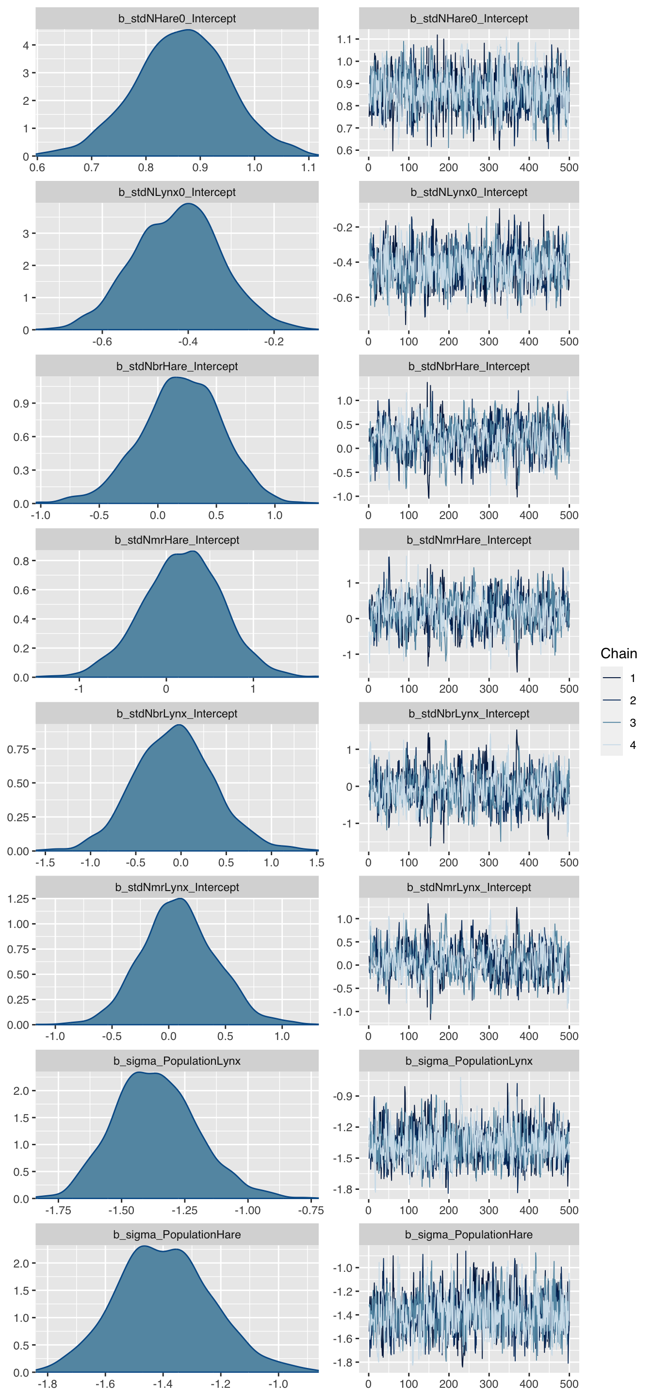
The charts look all sensible, but the parameters don’t look familiar, so let’s transform them back to the original scale.
trnf <- function(m, par, a, b){
  x <- as.vector(as_draws_matrix(m, par))
  tx <- a * exp(b * x)
  c(mean=mean(tx),
    se_mean = sd(tx)/sqrt(length(tx)),
    sd=sd(tx),
    quantile(tx, probs=c(0.025, 0.1, 0.5, 0.9, 0.975)))
}
round(rbind(
  Hare0 = trnf(mod, 'b_stdNHare0_Intercept', 10, 1),
  Lynx0 = trnf(mod, 'b_stdNLynx0_Intercept', 10, 1),
  brHare = trnf(mod, 'b_stdNbrHare_Intercept', 0.5, 0.25),
  mrHare = trnf(mod, 'b_stdNmrHare_Intercept', 0.025, 0.25),
  brLynx = trnf(mod, 'b_stdNbrLynx_Intercept', 0.025, 0.25),
  mrLynx = trnf(mod, 'b_stdNmrLynx_Intercept', 0.8, 0.25),
  SigmaHare = trnf(mod, 'b_sigma_PopulationHare', 1, 1),
  SigmaLynx = trnf(mod, 'b_sigma_PopulationLynx', 1, 1)
), 3)
## mean se_mean sd 2.5% 10% 50% 90% 97.5%
## Hare0 23.853 0.046 2.044 20.047 21.259 23.806 26.441 28.183
## Lynx0 6.578 0.015 0.659 5.376 5.741 6.567 7.426 7.970
## brHare 0.528 0.001 0.045 0.439 0.469 0.527 0.585 0.617
## mrHare 0.026 0.000 0.003 0.021 0.023 0.026 0.030 0.033
## brLynx 0.025 0.000 0.003 0.020 0.021 0.025 0.028 0.031
## mrLynx 0.821 0.002 0.069 0.700 0.738 0.817 0.913 0.967
## SigmaHare 0.251 0.001 0.043 0.182 0.202 0.247 0.307 0.350
## SigmaLynx 0.259 0.001 0.044 0.189 0.208 0.254 0.316 0.360Plot posterior simulations
Before I can draw simulations from the posterior predictive distributions, I have to expose the Stan functions to R.
expose_functions(mod, vectorize = TRUE, cacheDir = "~/Downloads/")Finally, I can run simulations from the posterior predictive model and compare the simulated output with the data.
library(tidybayes)
pred <- predicted_draws(mod, newdata = LH, n= 1000)
ggplot(pred, aes(x = Year, y = Pelts)) +
  stat_lineribbon(aes(y = .prediction),
                  .width = c(.99, .95, .8, .5),
                  color = "#08519C") +
  geom_point(data = pred) + labs(y="Pelts (thousands)") +
scale_fill_brewer() + facet_wrap(~ Population) 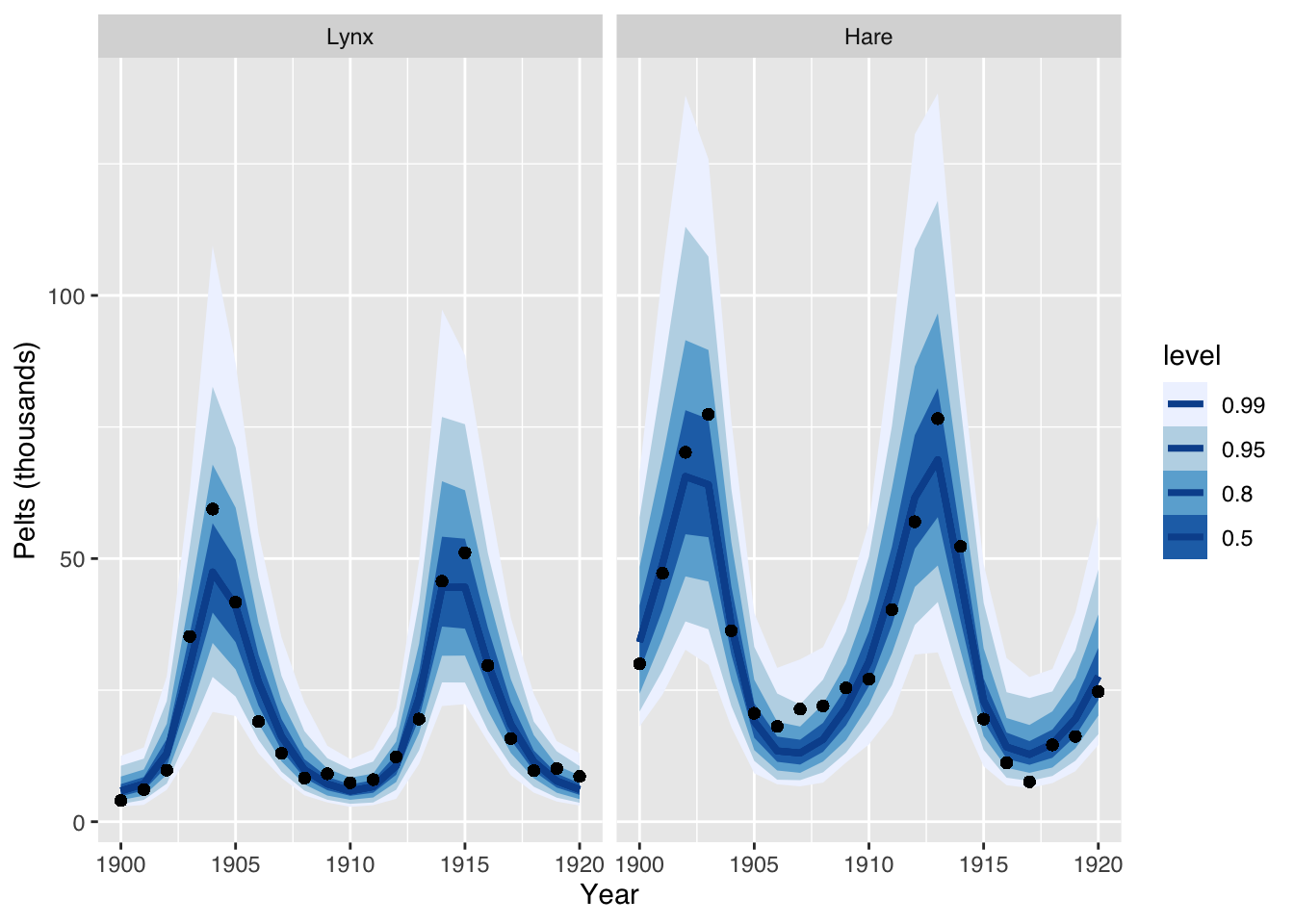
This plot suggests again that the model is a not unreasonable.
Summary
Although the model seems to describe the data well, it has its limitations:
- The solutions of the ODEs for a fixed set of parameters
are defined by the initial values, i.e. there are only stable orbits - No population can become extinct, i.e. if the initial value was greater 0
- There are many other factors impacting the birth and death rates of hares and lynxes apart from the interaction between the two populations
However, this example demonstrated how multivariate ODE models can
be fitted with brms. For more complex examples of multivariate ODEs
with brms see the case studies in section 5 of (Gesmann and Morris (2020)).
Session Info
session_info <- (sessionInfo()[-8])
utils:::print.sessionInfo(session_info, local=FALSE)
## R version 4.3.2 (2023-10-31)
## Platform: aarch64-apple-darwin20 (64-bit)
## Running under: macOS Sonoma 14.2.1
##
## Matrix products: default
## BLAS: /Library/Frameworks/R.framework/Versions/4.3-arm64/Resources/lib/libRblas.0.dylib
## LAPACK: /Library/Frameworks/R.framework/Versions/4.3-arm64/Resources/lib/libRlapack.dylib; LAPACK version 3.11.0
##
## attached base packages:
## NULL
##
## other attached packages:
## [1] tidybayes_3.0.6 cmdstanr_0.6.1.9000 brms_2.20.4
## [4] Rcpp_1.0.11 ggplot2_3.4.4 data.table_1.14.10
##
## loaded via a namespace (and not attached):
## [1] gridExtra_2.3 inline_0.3.19 rlang_1.1.2
## [4] magrittr_2.0.3 matrixStats_1.2.0 compiler_4.3.2
## [7] loo_2.6.0 vctrs_0.6.5 reshape2_1.4.4
## [10] stringr_1.5.1 arrayhelpers_1.1-0 pkgconfig_2.0.3
## [13] fastmap_1.1.1 backports_1.4.1 ellipsis_0.3.2
## [16] labeling_0.4.3 utf8_1.2.4 threejs_0.3.3
## [19] promises_1.2.1 rmarkdown_2.25 markdown_1.12
## [22] ps_1.7.5 purrr_1.0.2 xfun_0.41
## [25] cachem_1.0.8 jsonlite_1.8.8 highr_0.10
## [28] later_1.3.2 R6_2.5.1 dygraphs_1.1.1.6
## [31] RColorBrewer_1.1-3 bslib_0.6.1 stringi_1.8.3
## [34] StanHeaders_2.26.28 jquerylib_0.1.4 estimability_1.4.1
## [37] bookdown_0.37 rstan_2.32.3 knitr_1.45
## [40] zoo_1.8-12 base64enc_0.1-3 bayesplot_1.10.0
## [43] httpuv_1.6.13 Matrix_1.6-4 igraph_1.6.0
## [46] tidyselect_1.2.0 rstudioapi_0.15.0 abind_1.4-5
## [49] yaml_2.3.8 codetools_0.2-19 miniUI_0.1.1.1
## [52] blogdown_1.18 curl_5.2.0 processx_3.8.3
## [55] pkgbuild_1.4.3 lattice_0.22-5 tibble_3.2.1
## [58] plyr_1.8.9 shiny_1.8.0 withr_2.5.2
## [61] bridgesampling_1.1-2 posterior_1.5.0 coda_0.19-4
## [64] evaluate_0.23 RcppParallel_5.1.7 ggdist_3.3.1
## [67] xts_0.13.1 RcppEigen_0.3.3.9.4 pillar_1.9.0
## [70] tensorA_0.36.2.1 checkmate_2.3.1 DT_0.31
## [73] stats4_4.3.2 shinyjs_2.1.0 distributional_0.3.2
## [76] generics_0.1.3 rstantools_2.3.1.1 munsell_0.5.0
## [79] scales_1.3.0 gtools_3.9.5 xtable_1.8-4
## [82] glue_1.6.2 emmeans_1.9.0 tools_4.3.2
## [85] shinystan_2.6.0 colourpicker_1.3.0 mvtnorm_1.2-4
## [88] grid_4.3.2 tidyr_1.3.0 QuickJSR_1.0.9
## [91] crosstalk_1.2.1 colorspace_2.1-0 nlme_3.1-164
## [94] cli_3.6.2 svUnit_1.0.6 fansi_1.0.6
## [97] Brobdingnag_1.2-9 dplyr_1.1.4 V8_4.4.1
## [100] gtable_0.3.4 sass_0.4.8 digest_0.6.33
## [103] htmlwidgets_1.6.4 farver_2.1.1 htmltools_0.5.7
## [106] lifecycle_1.0.4 mime_0.12 shinythemes_1.2.0References
This post was motivated by question A. Solomon Kurz had for his bookdown project Statistical rethinking with brms, ggplot2, and the tidyverse: Second edition↩︎
Citation
For attribution, please cite this work as:Markus Gesmann (Feb 05, 2021) Fitting multivariate ODE models with brms. Retrieved from https://magesblog.com/post/2021-02-08-fitting-multivariate-ode-models-with-brms/
@misc{ 2021-fitting-multivariate-ode-models-with-brms,
author = { Markus Gesmann },
title = { Fitting multivariate ODE models with brms },
url = { https://magesblog.com/post/2021-02-08-fitting-multivariate-ode-models-with-brms/ },
year = { 2021 }
updated = { Feb 05, 2021 }
}