Hierarchical loss reserving with growth curves using brms
Ahead of the Stan Workshop on Tuesday,
here is another example of using brms (Bürkner (2017)) for claims reserving.
This time I will use a model inspired by the 2012 paper A Bayesian Nonlinear
Model for Forecasting Insurance Loss Payments (Zhang, Dukic, and Guszcza (2012)),
which can be seen as a follow-up to Jim Guszcza’s Hierarchical Growth Curve
Model (Guszcza (2008)).
I discussed Jim’s model in an earlier post
using Stan. Paul-Christian Bürkner showed then a little later how to implement this model using his brms package as part of the vignette Estimating Non-Linear Models with brms.
The Bayesian model proposed in (Zhang, Dukic, and Guszcza (2012)) predicts future claim payments across several insurance companies using growth curves.
The abstract of the paper motivates the model well:
“This approach enables us to carry out inference at the level of industry, company, and/or accident year, based on the full posterior distribution of all quantities of interest. In addition, prior experience and expert opinion can be incorporated into the analyses through judgmentally selected prior probability distributions.”
Data
Here is the data of the paper, which shows premiums and claim payments for 10 US insurance companies, for accidents years 1988 to 1997. In some cases the claims development is available for 10 years. The data itself is sourced from old regulatory filings.
library(data.table)
url <- "https://raw.githubusercontent.com/mages/diesunddas/master/Data/wc_data.csv"
WorkersComp <- fread(url, key=c("entity_name", "origin_year", "dev_year"))
WorkersComp <- WorkersComp[, loss_ratio := cumulative_paid/premium]
library(latticeExtra)
xyplot(loss_ratio*100 ~ dev_year | entity_name, groups = origin_year,
       data=WorkersComp, t="l", layout=c(5,2), as.table=TRUE,
       ylab="Loss ratio (%)", xlab="Dev year",
       main="Paid loss ratio developments by company and accident year",
       auto.key = list(space="top", columns=5),
       par.settings = theEconomist.theme(),
       scales = list(alternating=1))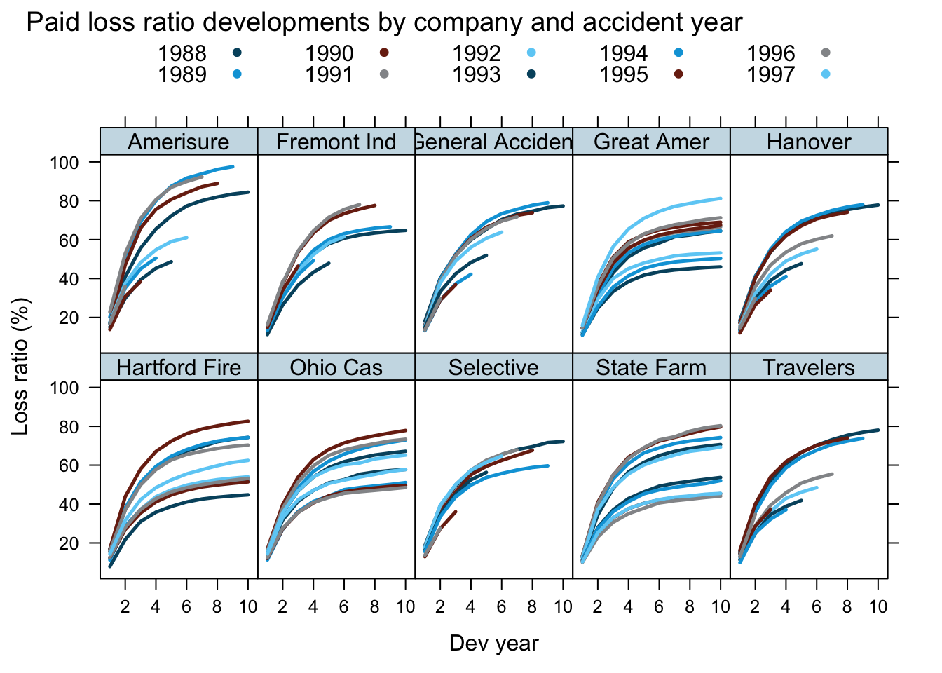
As usual, it is the aim to predict the future claims payments for the various accident years.
I will take a subset of the data to fit my model, and use the hold out data to review its performance.
For my training data set I will use data up to calendar year 1996, i.e. I exclude the 1997 accident year and future developments, ending up with triangles at the end of 1996.
WorkersComp[, loss_ratio_train := ifelse(dev_year + origin_year - 1 < 1997,
                                         loss_ratio, NA)]
Model
Growth curve
Growth curves are used to model the claims development process over time, see for example (Clark (2003)).
We can model the claims amount over time as: \[ \mbox{Paid claims}(t) = \mbox{Premiums} \cdot \gamma \cdot G(t) \] Here \(\gamma = \mbox{Ultimate paid claims} / \mbox{Premiums}\) represents the ultimate loss ratio (ULR) and \(G(t)\) a growth curve of cumulative paid claims to ultimate.
Alternatively, we can look at the loss ratio \(\ell(t) = \mbox{Paid claims}(t)/\mbox{Premiums}\) development:
\[ \ell(t) = \gamma \cdot G(t) \]
In this post I will use the loss ratio version, as it keeps the metrics around 1, regardless of the size of the insurance company.
There are many different options for growth curves (Panik (2014)). Here, following the paper (Zhang, Dukic, and Guszcza (2012)) I will also use the log-logistic curve:
\[ G(t; \theta, \omega, ) = \frac{t^{\omega}}{t^{\omega} + \theta^{\omega}} \]
growthcurve <- function(t, omega, theta) t^omega/(t^omega + theta^omega)
curve(growthcurve(x, 2, 4)*100, from = 0, to = 10, bty="n", ylim=c(0,100),
      main="Log-logistic gowth curve", ylab="% developed", xlab="Development period")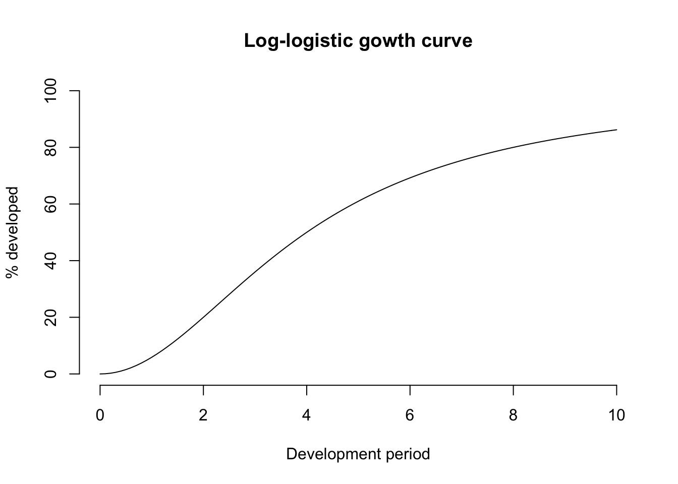
The growth curve parameter \(\theta\) corresponds to the time at which half of the growth has occurred, and the parameter \(\omega\) describes the slope of the curve around \(\theta\).
Hierarchical model
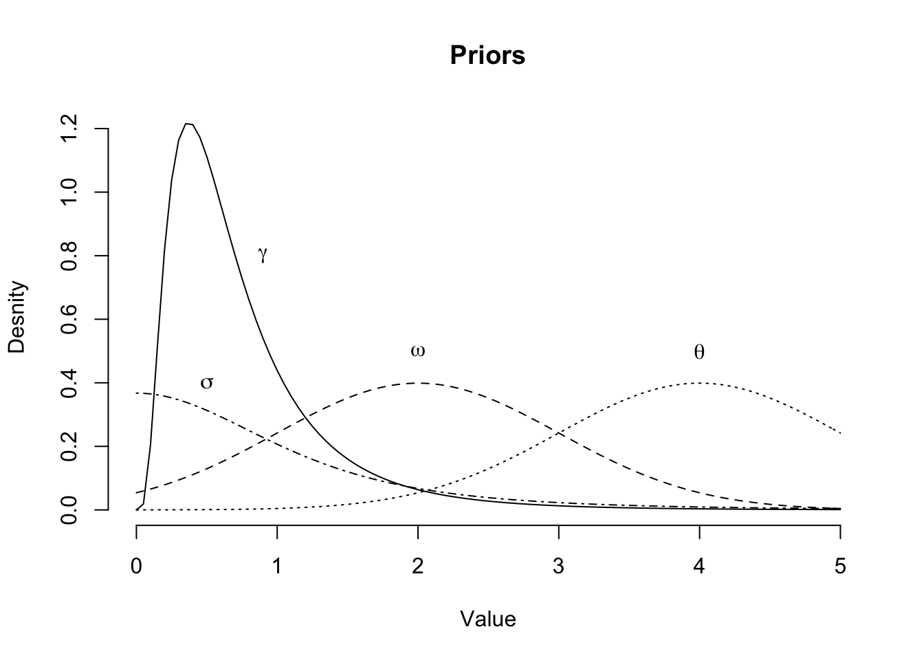
I shall assume that loss ratios follow a log-normal distribution, with the median described by growth curves to ultimate loss ratios. In addition, I believe that the ULRs and shapes of the growth curves are company \((k)\) specific and correlated, e.g. companies with lower ULRs have faster payment process; a lower value of \(\theta\), and a higher value of \(\omega\), but the ULR is expected to vary across accident years \((i)\) as well.
\[ \begin{aligned} \ell_{ik}(t) & \sim \log \mathcal{N}(\log{\mu_{ik}(t)}, \sigma^2) \\ \mu_{ik}(t) & = \gamma_{ik} \; G_k(t; \omega_k, \theta_k) \\ G_k(t; \omega_k, \theta_k) & = \frac{t^{\omega_k}}{t^{\omega_k} + \theta_k^{\omega_k}} \\ \gamma_{ik} & = \gamma + \gamma_k^0 + \gamma_{ik}^0\\ \omega_k & = \omega + \omega_k^0 \\ \theta_k & = \theta + \theta_k^0 \\ \mbox{Priors} & :\\ \gamma & \sim \log \mathcal{N}(\log(0.6), \log(2))\\ \theta & \sim \mathcal{N}(4, 1)^+ \\ \omega & \sim \mathcal{N}(2, 1)^+ \\ \sigma & \sim \mbox{Student-t}(3,0,1)^+\\ (\gamma_k^0, \omega_k^0, \theta_k^0) & \sim \mathcal{MN}\left(\mathbf{0}, \mathbf{\Sigma}\right) \\ \mathbf{\Sigma} & = \mathbf{D}(\sigma^0_{\gamma}, \sigma^0_{\omega}, \sigma^0_{\theta})\, \mathbf{\Omega}\,\mathbf{D}(\sigma^0_{\gamma}, \sigma^0_{\omega}, \sigma^0_{\theta})\\ \sigma^0_{\gamma}, \sigma^0_{\omega}, \sigma^0_{\theta}& \sim \mbox{Student-t}(3, 0, 1)^+\\ \mathbf{\Omega} & \sim \mbox{LKJ}(2) \\ \gamma_{ik}^0 & \sim \mathcal{N}(0, \sigma^2_{[ik]})\\ \sigma_{[ik]} & \sim \mbox{Student-t}(3,0,1)^+ \\ \end{aligned} \]
 This model is similar to the one proposed in (Zhang, Dukic, and Guszcza (2012)), but there are some differences:
- loss ratios are modelled instead of loss amounts,
- \(\sigma\) is kept constant across all companies \(k\),
- \(\gamma_k^0, \omega_k^0, \theta_k^0\) are modelled via a multivariate normal, instead of a log-normal distribution,
- the prior for \(\Omega\) is assumed to be a \(LKJ\) instead of an inverse-Wishart distribution,
- \(\gamma_{ik}^0\) are modelled additive and drawn from a normal, instead of log-normal distribution,
- there is no auto-regressive process,
- development years are used instead of development months.
Hopefully, all of the above changes have little impact on the model performance, but will make the use of brm easier/ possible.
Fitting the model
First I load the relevant R packages.
library(rstan)
rstan_options(auto_write = TRUE)
options(mc.cores = parallel::detectCores())
library(brms)
Next I specify the non-linear hierarchical model and set my prior distributions.
To allow for interaction between companies and accident years I use the “:” operator,
additionally I add ID as a place holder to model the group effect of entity_name
on ulr, omega and theta and to allow for correlation at company level. For more details see (Bürkner (2017)).
frml <- bf(loss_ratio_train ~ log(ulr * dev_year^omega/(dev_year^omega + theta^omega)),
           ulr ~ 1 +  (1|ID|entity_name) + (1|origin_year:entity_name) ,
           omega ~ 1 + (1|ID|entity_name),
           theta ~ 1 + (1|ID|entity_name),
           nl = TRUE)

my_priors <- c(
  prior(lognormal(log(0.6), log(2)), nlpar = "ulr", lb=0),
  prior(normal(2, 1), nlpar = "omega", lb=0),
  prior(normal(4, 1), nlpar = "theta", lb=0),
  prior(student_t(3, 0, 1), class = "sigma"),
  prior(student_t(3, 0, 1), class = "sd", nlpar = "omega"),
  prior(student_t(3, 0, 1), class = "sd", nlpar = "theta"),
  prior(student_t(3, 0, 1), class = "sd", nlpar = "ulr"),
  prior(lkj(2), class="cor"))

mdl <- brm(frml, data = WorkersComp, prior = my_priors, seed = 1234,
           family = lognormal(link = "identity", link_sigma = "identity"),
           control = list(adapt_delta = 0.999, max_treedepth=15))
Get yourself a cup of tea, as the sampling takes about 15 - 30 minutes, depending on your computer
Model review
Let’s look at the output of brm.
mdl## Family: lognormal
## Links: mu = identity; sigma = identity
## Formula: loss_ratio_train ~ log(ulr * dev_year^omega/(dev_year^omega + theta^omega))
## ulr ~ 1 + (1 | ID | entity_name) + (1 | origin_year:entity_name)
## omega ~ 1 + (1 | ID | entity_name)
## theta ~ 1 + (1 | ID | entity_name)
## Data: WorkersComp (Number of observations: 450)
## Samples: 4 chains, each with iter = 2000; warmup = 1000; thin = 1;
## total post-warmup samples = 4000
##
## Group-Level Effects:
## ~entity_name (Number of levels: 10)
## Estimate Est.Error l-95% CI u-95% CI Rhat
## sd(ulr_Intercept) 0.05 0.03 0.01 0.11 1.00
## sd(omega_Intercept) 0.12 0.04 0.06 0.22 1.00
## sd(theta_Intercept) 0.11 0.05 0.05 0.23 1.00
## cor(ulr_Intercept,omega_Intercept) -0.13 0.34 -0.75 0.54 1.00
## cor(ulr_Intercept,theta_Intercept) 0.24 0.35 -0.53 0.81 1.00
## cor(omega_Intercept,theta_Intercept) 0.08 0.31 -0.52 0.68 1.00
## Bulk_ESS Tail_ESS
## sd(ulr_Intercept) 530 640
## sd(omega_Intercept) 2897 3218
## sd(theta_Intercept) 1933 2591
## cor(ulr_Intercept,omega_Intercept) 1891 1896
## cor(ulr_Intercept,theta_Intercept) 2315 2512
## cor(omega_Intercept,theta_Intercept) 3778 2814
##
## ~origin_year:entity_name (Number of levels: 90)
## Estimate Est.Error l-95% CI u-95% CI Rhat Bulk_ESS Tail_ESS
## sd(ulr_Intercept) 0.11 0.01 0.10 0.13 1.00 1150 1829
##
## Population-Level Effects:
## Estimate Est.Error l-95% CI u-95% CI Rhat Bulk_ESS Tail_ESS
## ulr_Intercept 0.71 0.02 0.66 0.75 1.00 2853 2263
## omega_Intercept 1.82 0.04 1.73 1.91 1.00 3536 2908
## theta_Intercept 2.12 0.04 2.04 2.22 1.00 3954 2702
##
## Family Specific Parameters:
## Estimate Est.Error l-95% CI u-95% CI Rhat Bulk_ESS Tail_ESS
## sigma 0.03 0.00 0.03 0.04 1.00 3369 2894
##
## Samples were drawn using sampling(NUTS). For each parameter, Bulk_ESS
## and Tail_ESS are effective sample size measures, and Rhat is the potential
## scale reduction factor on split chains (at convergence, Rhat = 1).The output looks promising, particularly for ulr, omega and theta. The estimators are very similar to the ones published in (Zhang, Dukic, and Guszcza (2012)).
Perhaps, the correlation term is not relevant, given the wide credible intervals. However, the positive correlation between ULR and \(\theta\) (higher ULR correlates with longer claims settlement process) was expected, equally a negative correlation between ULR and \(\omega\) looks sensible.
plot(mdl)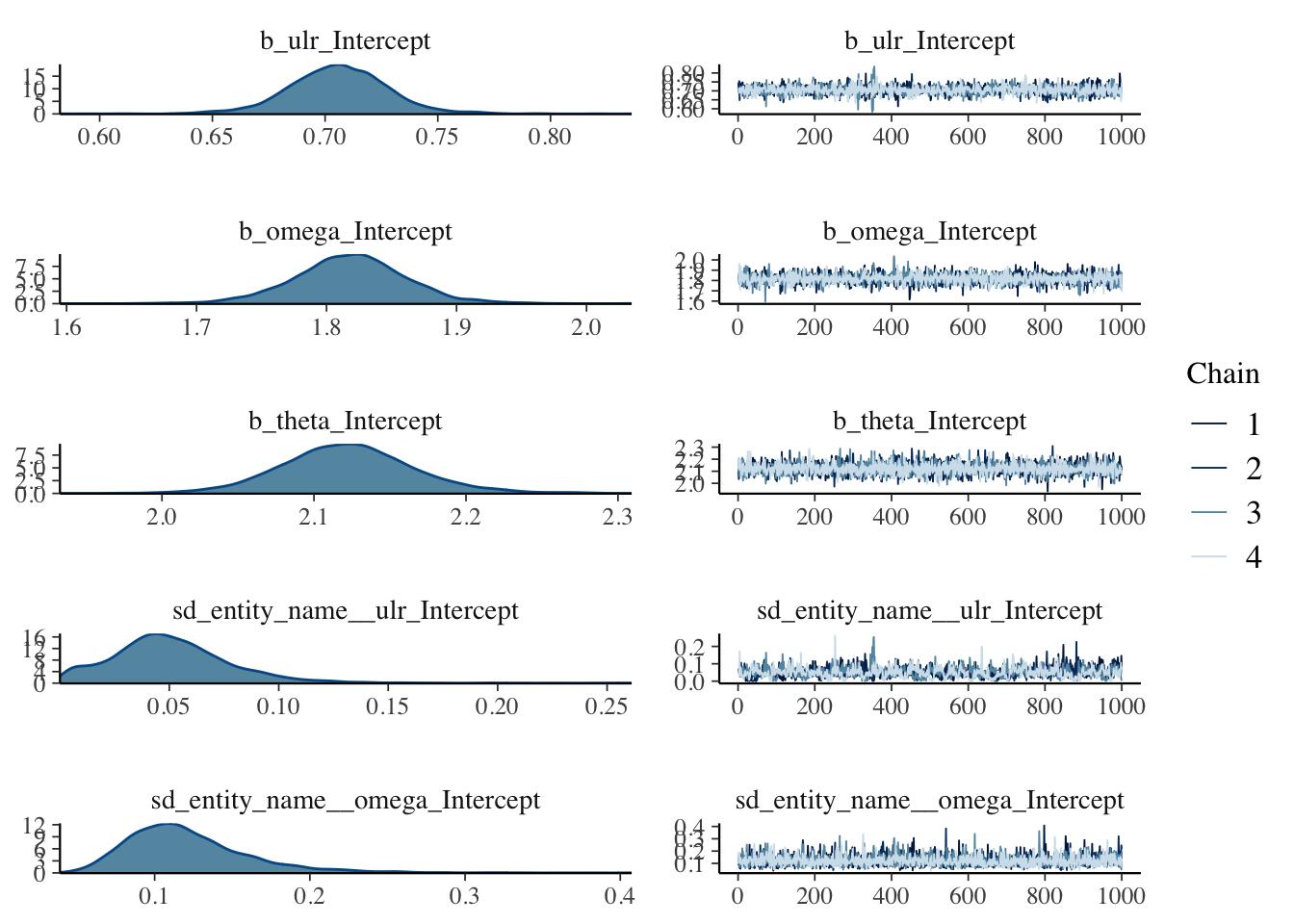
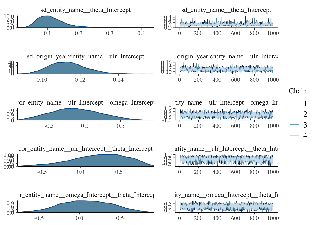
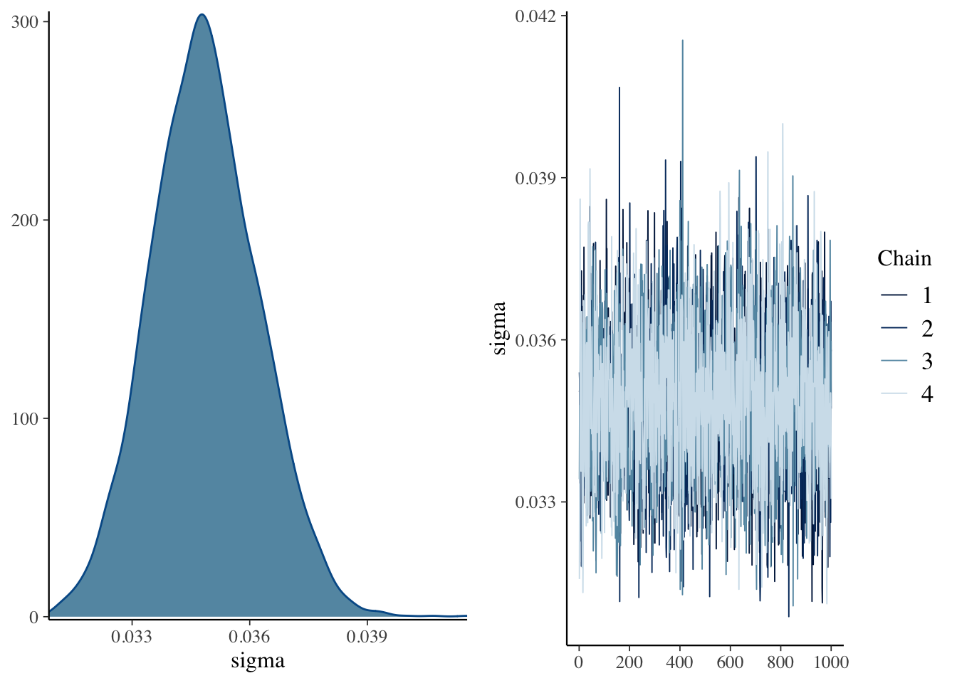
The plots don’t show anything that raise concerns on my side.
Thus, let’s move on to something more interesting. I’d like to compare the estimated parameters \(\gamma_k\) for the ULRs across companies.
library(bayesplot)
theme_update(text = element_text(family = "sans"))
posterior <- as.array(mdl)
mcmc_areas(
   posterior,
   pars = names(mdl$fit)[c(1, 12:21)],
   prob = 0.8, # 80% intervals
   prob_outer = 0.99, # 99%
   point_est = "mean"
) + ggplot2::labs(
  title = "ULR posterior distributions",
  subtitle = "with medians and 80% intervals"
)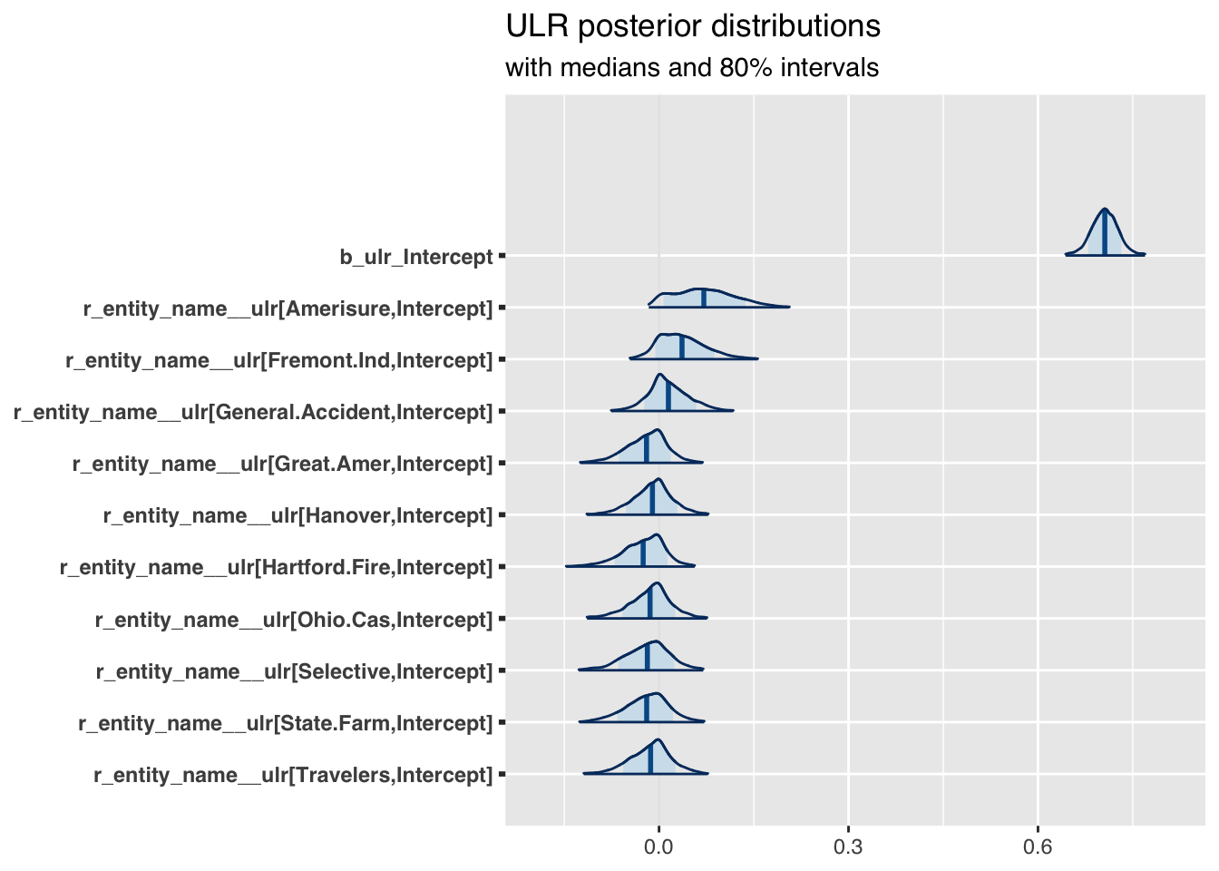
Now this is interesting! For the industry the expected URL is around 70% across all years. However, the chart shows as well how the companies vary from the industry in an additive way. Companies with a distribution left of \(0\) are likely to out-perform the industry, while companies to the right of \(0\) are likely under-performers.
Model prediction
Let’s use our model to predict future claims up to 1997 and shows also the 2.5%ile and 97.5%ile of the posterior predictive distribution.
What I really like about this model is that I can also make a prediction for the 1997 accident year, although I used only data up to 1996. The model estimated for each company the “average” development pattern and ULR, which can be used to give us an initial view for the 1997 accident year - basically a sensible planning assumption, based on past experience.
n_dev_years <- max(WorkersComp$dev_year)
n_entities <- length(unique(WorkersComp$entity_name))
n_origin_years <- length(unique(WorkersComp$origin_year))
newdat <- data.table(
  entity_name = rep(unique(WorkersComp$entity_name), each=n_origin_years * n_dev_years),
  origin_year = rep(unique(WorkersComp$origin_year), n_entities * n_dev_years),
  dev_year = rep(rep(c(1:n_dev_years), n_entities), each=n_origin_years),
  key = c("entity_name", "origin_year", "dev_year"))

pp <- posterior_predict(mdl, newdata = newdat, allow_new_levels=TRUE)
plotData <- WorkersComp[newdat]
plotData$PredLR <- apply(pp, 2, mean)
plotData$PredLR25 <- apply(pp, 2, quantile, probs=0.025)
plotData$PredLR975 <- apply(pp, 2, quantile, probs=0.975)
plotData$loss_ratio_test <- WorkersComp[plotData]$loss_ratio
To visualise the output I use a function from an earlier post.
plotDevBananas(PredLR25*100 + PredLR975*100 + PredLR*100 +
                 loss_ratio_train*100 + loss_ratio_test*100 ~
                 dev_year |  factor(origin_year) * entity_name,
               data=plotData[order(origin_year, dev_year)],  main="")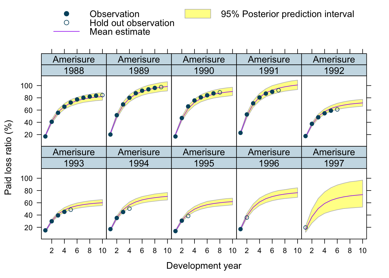
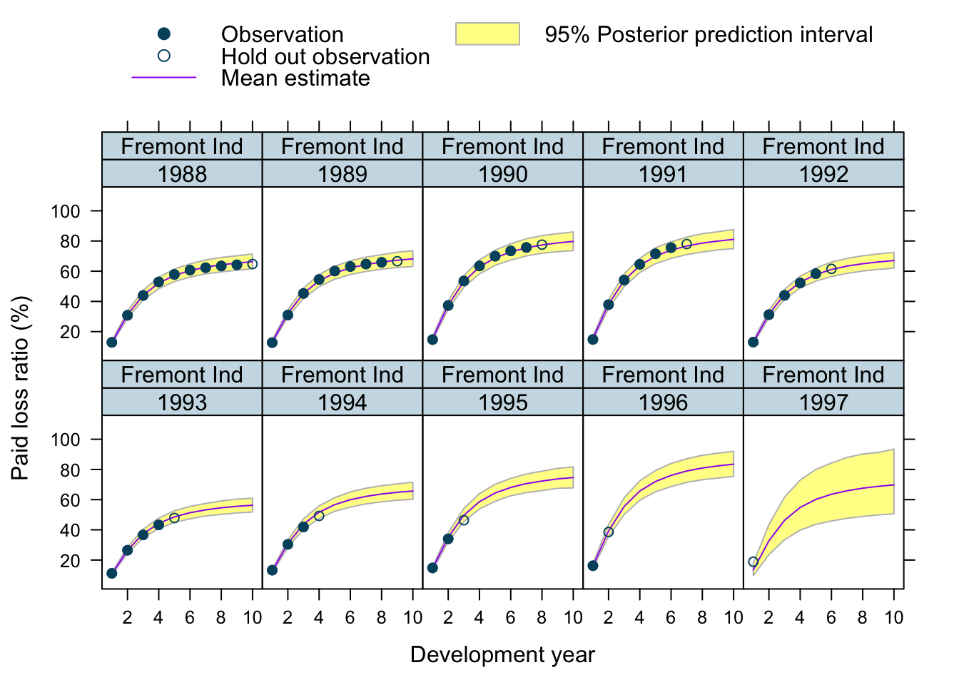
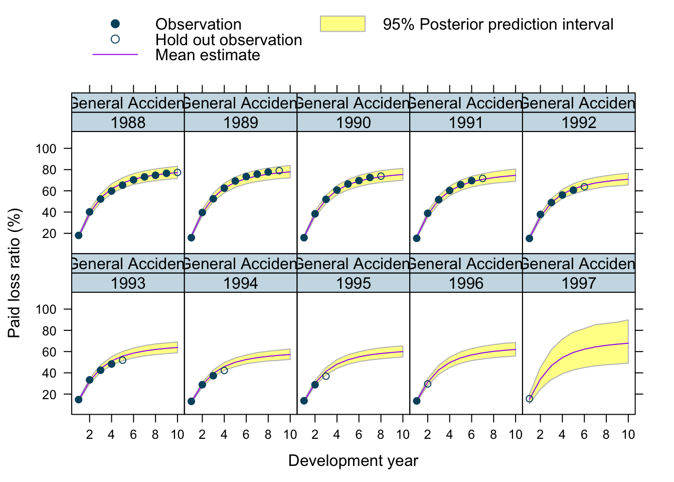
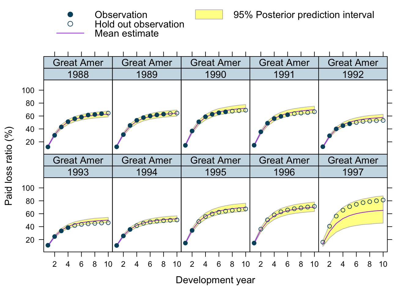
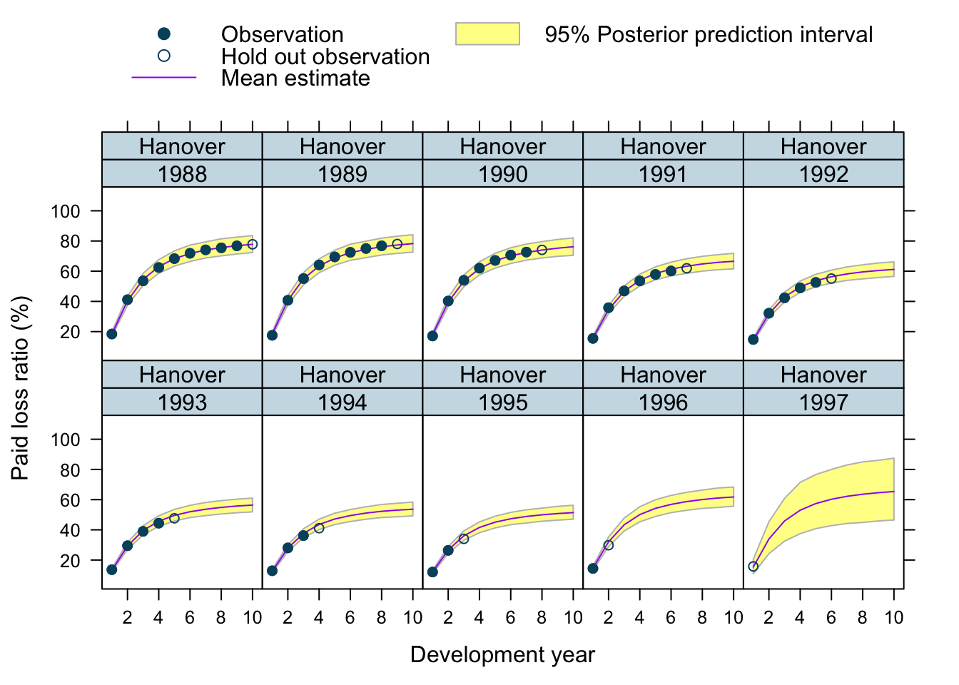
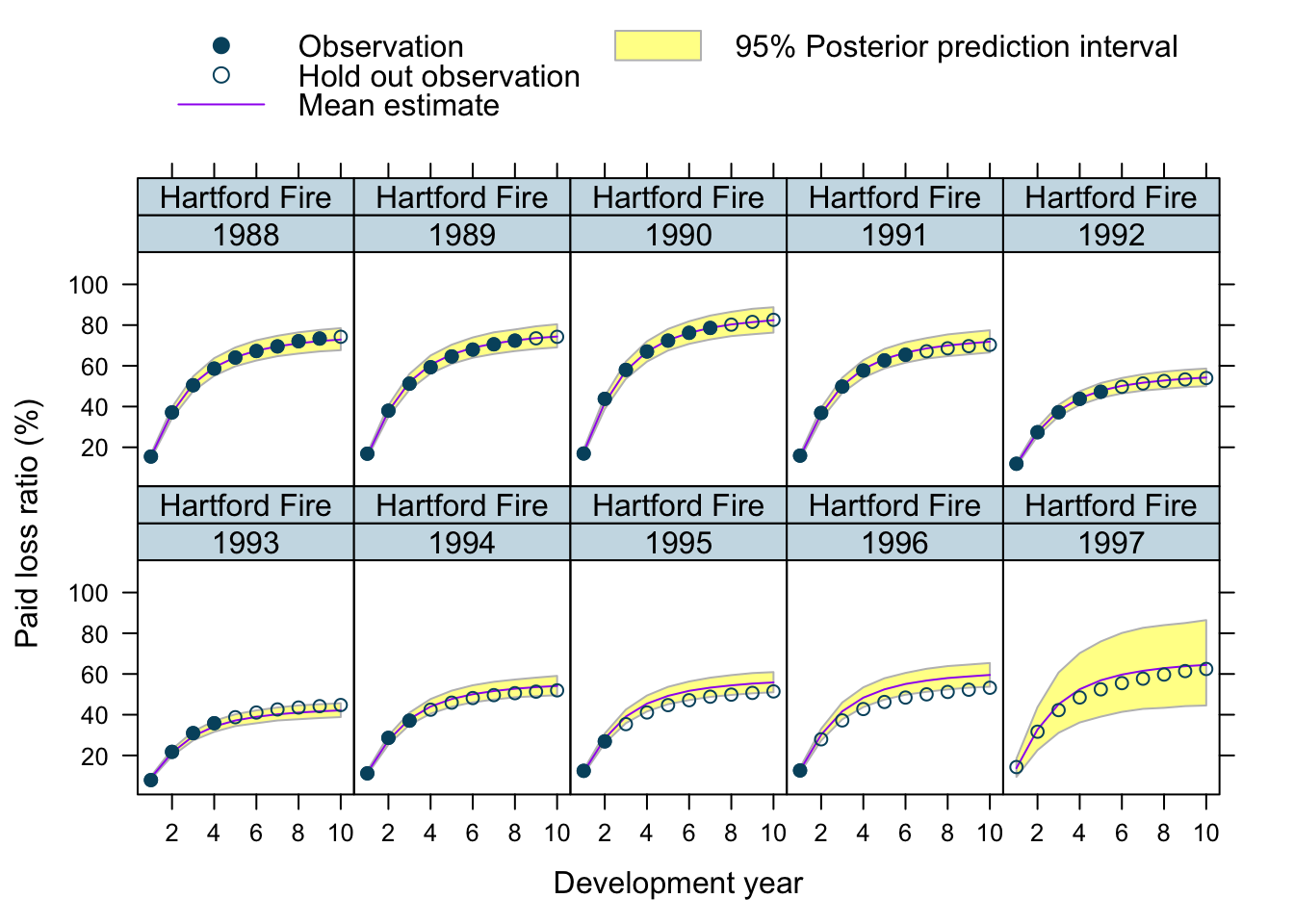
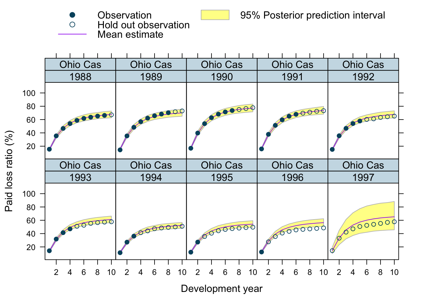
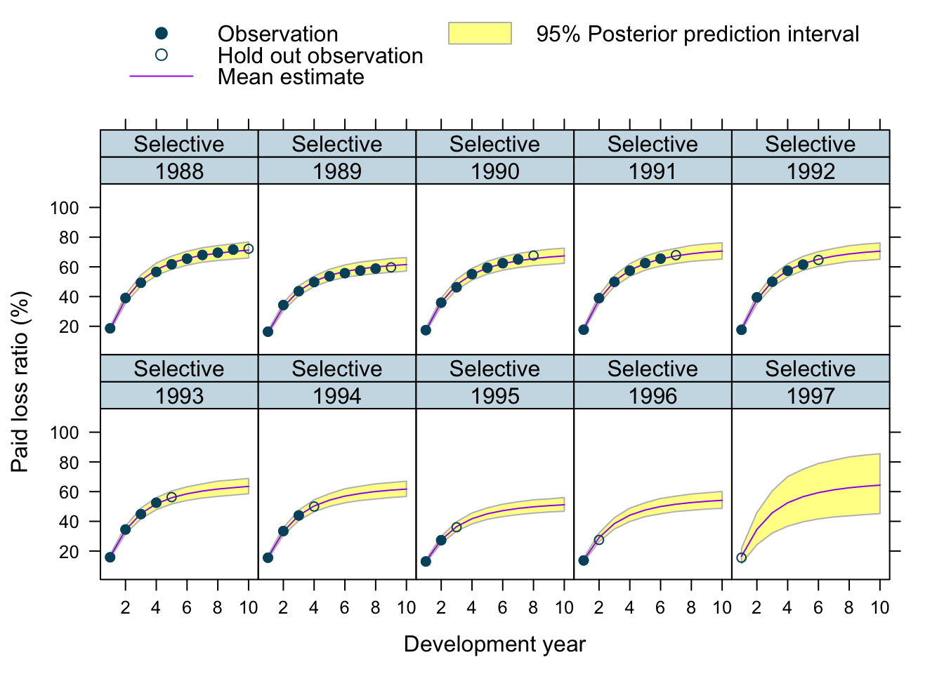

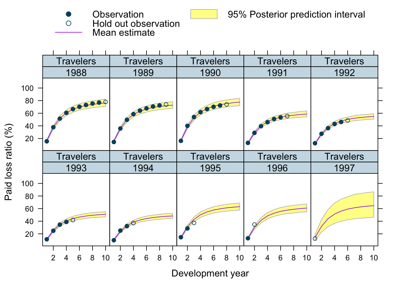
Observations
Overall, I am very happy with the predictions and the plots. The more recent accident years have a wider development funnel, as we have less data available.
The actual performance of the 1997 accident year looks a little peculiar. The recorded loss ratios for Great Amer is much worse than predicted, the loss ratios for Hartford Fire, Ohio Cas and most significantly for State Farm performed better than expected. Indeed, all 3 of them seem to have improved their performance from 1995 onwards.
Conclusions
Modelling several companies at the same time can be a powerful approach to incorporate more data into the reserving process. The model shown here not only predicted future claims, but as a by-product ULRs by company and for the industry. Further, it allowed me to make an initial prediction for future accident years, which can be helpful for business planning and pricing.
Using parametric growth curves can provide a robust approach to model the claims process and avoids the selection of tail factors in traditional reserving methods, such as chain-ladder.
Motivating growth curves via differential equations might be an appropriate step to take. I really like Jake Morris’ approach of hierarchical compartmental models for loss reserving (Morris (2016)), which I outlined in an earlier post. It highlights the value of developing an understanding of the data generating process.
Finally, one can take the generated Stan code of brm, use stancode(mdl) to access it, to create even more sophisticated models than I have shown here.
You can find further articles on claims reserving on my blog.
Update
Jake and I published a new research paper on Hierarchical Compartmental Reserving Models:

Gesmann, M., and Morris, J. “Hierarchical Compartmental Reserving Models.” Casualty Actuarial Society, CAS Research Papers, 19 Aug. 2020, https://www.casact.org/sites/default/files/2021-02/compartmental-reserving-models-gesmannmorris0820.pdf
Session Info
sessionInfo()## R version 4.0.3 (2020-10-10)
## Platform: x86_64-apple-darwin17.0 (64-bit)
## Running under: macOS Big Sur 10.16
##
## Matrix products: default
## BLAS: /Library/Frameworks/R.framework/Versions/4.0/Resources/lib/libRblas.dylib
## LAPACK: /Library/Frameworks/R.framework/Versions/4.0/Resources/lib/libRlapack.dylib
##
## locale:
## [1] en_GB.UTF-8/en_GB.UTF-8/en_GB.UTF-8/C/en_GB.UTF-8/en_GB.UTF-8
##
## attached base packages:
## [1] stats graphics grDevices utils datasets methods base
##
## other attached packages:
## [1] brms_2.14.4 Rcpp_1.0.5 rstan_2.21.2
## [4] ggplot2_3.3.3 StanHeaders_2.21.0-7 latticeExtra_0.6-29
## [7] lattice_0.20-41 data.table_1.13.6
##
## loaded via a namespace (and not attached):
## [1] minqa_1.2.4 colorspace_2.0-0 ellipsis_0.3.1
## [4] ggridges_0.5.2 rsconnect_0.8.16 markdown_1.1
## [7] base64enc_0.1-3 DT_0.16 fansi_0.4.1
## [10] mvtnorm_1.1-1 codetools_0.2-18 bridgesampling_1.0-0
## [13] splines_4.0.3 knitr_1.30 shinythemes_1.1.2
## [16] bayesplot_1.7.2 projpred_2.0.2 jsonlite_1.7.2
## [19] nloptr_1.2.2.2 png_0.1-7 shiny_1.5.0
## [22] compiler_4.0.3 backports_1.2.1 assertthat_0.2.1
## [25] Matrix_1.3-0 fastmap_1.0.1 cli_2.2.0
## [28] later_1.1.0.1 htmltools_0.5.0 prettyunits_1.1.1
## [31] tools_4.0.3 igraph_1.2.6 coda_0.19-4
## [34] gtable_0.3.0 glue_1.4.2 reshape2_1.4.4
## [37] dplyr_1.0.2 V8_3.4.0 vctrs_0.3.6
## [40] nlme_3.1-151 blogdown_0.21 crosstalk_1.1.0.1
## [43] xfun_0.19 stringr_1.4.0 ps_1.5.0
## [46] lme4_1.1-26 mime_0.9 miniUI_0.1.1.1
## [49] lifecycle_0.2.0 gtools_3.8.2 statmod_1.4.35
## [52] MASS_7.3-53 zoo_1.8-8 scales_1.1.1
## [55] colourpicker_1.1.0 promises_1.1.1 Brobdingnag_1.2-6
## [58] parallel_4.0.3 inline_0.3.17 shinystan_2.5.0
## [61] RColorBrewer_1.1-2 gamm4_0.2-6 yaml_2.2.1
## [64] curl_4.3 gridExtra_2.3 loo_2.4.1
## [67] stringi_1.5.3 dygraphs_1.1.1.6 boot_1.3-25
## [70] pkgbuild_1.2.0 rlang_0.4.10 pkgconfig_2.0.3
## [73] matrixStats_0.57.0 evaluate_0.14 purrr_0.3.4
## [76] rstantools_2.1.1 htmlwidgets_1.5.3 tidyselect_1.1.0
## [79] processx_3.4.5 plyr_1.8.6 magrittr_2.0.1
## [82] bookdown_0.21 R6_2.5.0 generics_0.1.0
## [85] pillar_1.4.7 withr_2.3.0 mgcv_1.8-33
## [88] xts_0.12.1 abind_1.4-5 tibble_3.0.4
## [91] crayon_1.3.4 rmarkdown_2.6 jpeg_0.1-8.1
## [94] grid_4.0.3 callr_3.5.1 threejs_0.3.3
## [97] digest_0.6.27 xtable_1.8-4 httpuv_1.5.4
## [100] RcppParallel_5.0.2 stats4_4.0.3 munsell_0.5.0
## [103] shinyjs_2.0.0References
Citation
For attribution, please cite this work as:Markus Gesmann (Jul 15, 2018) Hierarchical loss reserving with growth curves using brms. Retrieved from https://magesblog.com/post/2018-07-15-hierarchical-loss-reserving-with-growth-cruves-using-brms/
@misc{ 2018-hierarchical-loss-reserving-with-growth-curves-using-brms,
author = { Markus Gesmann },
title = { Hierarchical loss reserving with growth curves using brms },
url = { https://magesblog.com/post/2018-07-15-hierarchical-loss-reserving-with-growth-cruves-using-brms/ },
year = { 2018 }
updated = { Jul 15, 2018 }
}