Loss Developments via Growth Curves and Stan

Last week I posted a biological example of fitting a non-linear growth curve with Stan/RStan. Today, I want to apply a similar approach to insurance data using ideas by David Clark [1] and James Guszcza [2].

Instead of predicting the growth of dugongs (sea cows), I would like to predict the growth of cumulative insurance loss payments over time, originated from different origin years. Loss payments of younger accident years are just like a new generation of dugongs, they will be small in size initially, grow as they get older, until the losses are fully settled.

Here is my example data set:

library(ChainLadder)
round(GenIns/1000)

##       dev
## origin   1    2    3    4    5    6    7    8    9   10
##     1  358 1125 1735 2218 2746 3320 3466 3606 3834 3901
##     2  352 1236 2170 3353 3799 4120 4648 4914 5339   NA
##     3  291 1292 2219 3235 3986 4133 4629 4909   NA   NA
##     4  311 1419 2195 3757 4030 4382 4588   NA   NA   NA
##     5  443 1136 2128 2898 3403 3873   NA   NA   NA   NA
##     6  396 1333 2181 2986 3692   NA   NA   NA   NA   NA
##     7  441 1288 2420 3483   NA   NA   NA   NA   NA   NA
##     8  359 1421 2864   NA   NA   NA   NA   NA   NA   NA
##     9  377 1363   NA   NA   NA   NA   NA   NA   NA   NA
##     10 344   NA   NA   NA   NA   NA   NA   NA   NA   NA

plot(GenIns/1000, lattice=TRUE, 
     layout=c(5,2), pch=19, cex=0.5, 
     main="Cumulative development by origin year")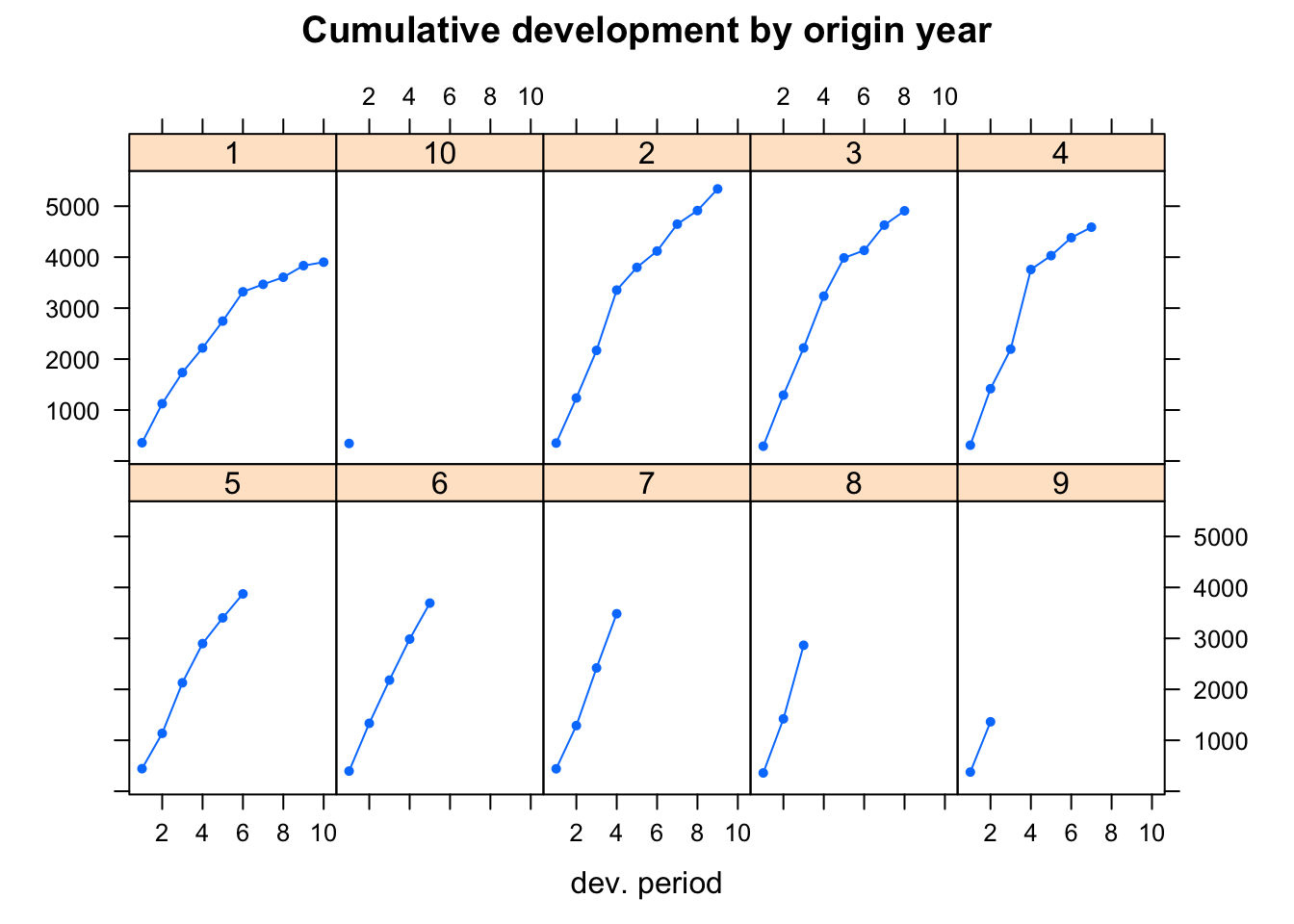

Following the articles cited above I will assume that the growth can be explained by a Weibull curve, with two parameters \(\theta\) (scale) and \(\omega\) (shape): \[ G(dev|\omega, \theta) = 1 - \exp\left(-\left(\frac{dev}{\theta}\right)^\omega\right) \]

Inspired by the classical over-dispersed Poisson GLM in actuarial science, Guszcza [2] assumes a power variance structure for the process error as well. For the purpose of this post I will assume that claims cost follow a Normal distribution, to make a comparison with a the classical least square regression easier. With a prior estimate of the ultimate claims cost the cumulative loss can be modelled as:

\[ \begin{aligned} CL_{AY, dev} & \sim \mathcal{N}(\mu_{dev}, \sigma^2_{dev})\\ \mu_{dev} & = Ult \cdot G(dev|\omega, \theta)\\ \sigma_{dev} & = \sigma \sqrt{\mu_{dev}} \end{aligned} \]

Perhaps, the above formula suggests a hierarchical modelling approach, with different ultimate loss costs by accident year. Indeed, this is the focus of [2] and I will endeavour to reproduce the results with Stan in my next post, but today I will stick to a pooled model that assumes a constant ultimate loss across all accident years, i.e. \(Ult_{AY} = Ult \;\forall\; AY\).

To prepare my analysis I read in the data as a long data frame instead of the matrix structure above. Additionally, I compose another data frame that I will use later to predict payments two years beyond the first 10 years. Furthermore, to align the output with [2] I relabelled the development periods from years to months, so that year 1 becomes month 6, year 2 becomes month 18, etc. The accident years run from 1991 to 2000, while the variable origin maps those years from 1 to 10.

# Read data as long table
url <- "https://raw.githubusercontent.com/mages/diesunddas/master/Data/ClarkTriangle.csv"
dat <- read.csv(url)
dat$origin <- dat$AY-min(dat$AY)+1
dat <- dat[order(dat$dev),]
# Add future dev years
nyears <- 12
newdat <- data.frame(
  origin=rep(1:10, each=nyears),
  AY=rep(sort(unique(dat$AY)), each=nyears),  
  dev=rep(seq(from=6, to=nyears*12-6, by=12), 10)
)
newdat <- merge(dat, newdat, all=TRUE)
newdat <- newdat[order(newdat$dev),]

To get a reference point for Stan I start with a non-linear least square regression:

## Pooled regression
start.vals <- c(ult = 5000, omega = 1.4, theta = 45)
library(nlme)
w0 <- gnls(cum ~ ult*(1 - exp(-(dev/theta)^omega)),
           weights = varPower(fixed=.5),
           data=dat, start = start.vals)
w0

## Generalized nonlinear least squares fit
##   Model: cum ~ ult * (1 - exp(-(dev/theta)^omega)) 
##   Data: dat 
##   Log-likelihood: -389.072
## 
## Coefficients:
##         ult       omega       theta 
## 4642.641548    1.349402   40.054344 
## 
## Variance function:
##  Structure: Power of variance covariate
##  Formula: ~fitted(.) 
##  Parameter estimates:
## power 
##   0.5 
## Degrees of freedom: 55 total; 52 residual
## Residual standard error: 6.711733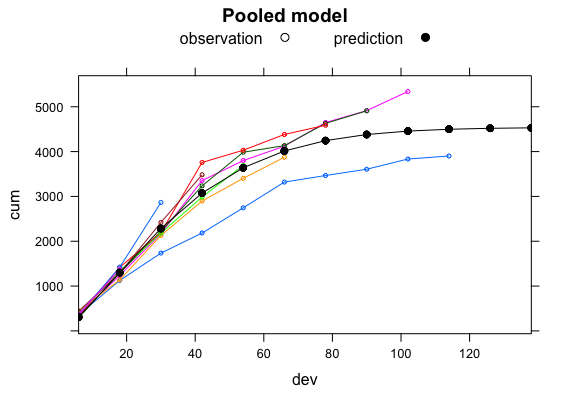

The output above doesn’t look unreasonable, apart from the accident years 1991, 1992 and 1998. The output of gnls gives me an opportunity to provide my prior distributions with good starting points. I will use an inverse Gamma as a prior for \(\sigma\), constrained Normals for the parameters \(\theta, \omega\) and \(Ult\) as well. If you have better ideas, then please get in touch.

The Stan code below is very similar to last week. Again, I am interested here in the posterior distributions, hence I add a block to generate quantities from those. Note, Stan comes with a build-in function for the cumulative Weibull distribution weibull_cdf.

stanmodel <-
"data {
  int<lower=0> N; // total number of rows
  real cum[N]; // cumulative paid
  real dev[N]; // development period
  // Variables for predictions
  int<lower=0> new_N; // number of rows of prediction data set
  real new_dev[new_N]; // development periods to predict
}
parameters {
  real<lower=0> theta; // scale parameter
  real<lower=0> omega; // shape parameter 
  real<lower=0> ult; // ultimate loss
  real<lower=0> tau; // model precession
}
transformed parameters {
  real sigma; // process error
  sigma = 1 / sqrt(tau);
}
model {
  real mu[N];
  real disp_sigma[N];
  // Priors
  theta ~ normal(46, 10); // scale parameter
  omega ~ normal(1.4, 1); // shape parameter
  tau ~ gamma(.0001, .0001);
  ult ~ normal(5000, 1000);  
  // Hyperparameters: Modelled parameters
  for (i in 1:N){
    mu[i] <- ult * weibull_cdf(dev[i], omega, theta);
    disp_sigma[i] = sigma * sqrt(mu[i]);
  }
  // Likelihood: Modelled data
  cum ~ normal(mu, disp_sigma); 
}
generated quantities{
  real Y_mean[new_N];
  real Y_pred[new_N];
  for(i in 1:new_N){
    // Posterior parameter distribution of the mean
    Y_mean[i] = ult * weibull_cdf(new_dev[i], omega, theta);
    // Posterior predictive distribution
    Y_pred[i] = normal_rng(Y_mean[i], sigma*sqrt(Y_mean[i]));   
  }
}"
cat(stanmodel, file="Pooled_Model_for_Loss_Reserving.stan")

I store the Stan code in a separate text file, which I read into R to compile the model. The compilation takes a little time. The sampling itself is done in a few seconds.

Let’s take a look at the output:

library(rstan)
rstan_options(auto_write = TRUE)
options(mc.cores = parallel::detectCores()) 
pooledDso <- stan_model(file = "Pooled_Model_for_Loss_Reserving.stan",
                        model_name = "GrowthCurve")
fit <- sampling(pooledDso, iter=5500, warmup=500,
                thin=2, cores=2, chains=4, seed=1037025002,
                data = list(N = nrow(dat),
                            cum=dat$cum,
                            dev=dat$dev,
                            new_N=nrow(newdat),
                            new_dev=newdat$dev))

print(fit, pars=c("ult", "omega", "theta", "sigma"),
      probs=c(0.5, 0.75, 0.95))

## Inference for Stan model: GrowthCurve.
## 4 chains, each with iter=5500; warmup=500; thin=2; 
## post-warmup draws per chain=2500, total post-warmup draws=10000.
## 
##          mean se_mean     sd     50%     75%     95% n_eff Rhat
## ult   4758.39    3.10 242.73 4739.08 4900.08 5186.92  6146    1
## omega    1.35    0.00   0.07    1.35    1.40    1.47  6743    1
## theta   41.74    0.05   3.51   41.45   43.75   47.96  5928    1
## sigma    6.83    0.01   0.68    6.77    7.25    8.04  8027    1
## 
## Samples were drawn using NUTS(diag_e) at Sun Aug 16 08:58:26 2020.
## For each parameter, n_eff is a crude measure of effective sample size,
## and Rhat is the potential scale reduction factor on split chains (at 
## convergence, Rhat=1).

rstan::traceplot(fit, pars=c("ult", "omega", "theta", "sigma"))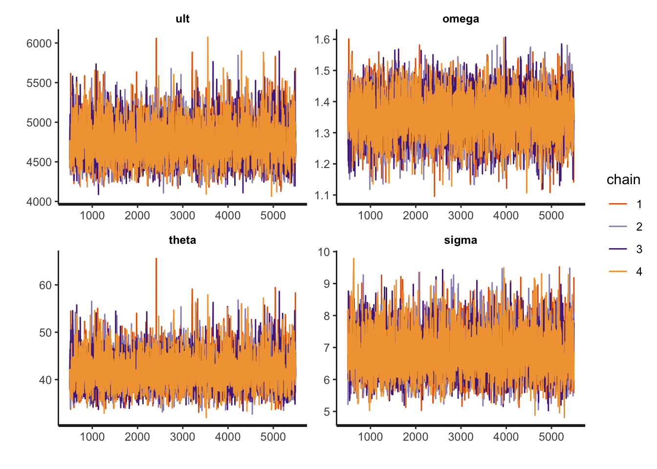

stan_dens(fit, pars=c("ult", "omega", "theta", "sigma"), 
          fill="skyblue")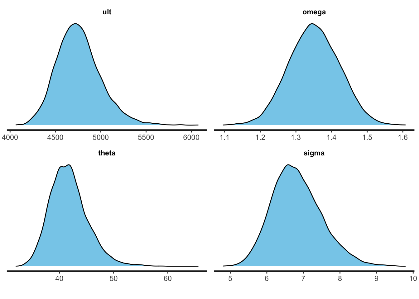

The parameters are a little different to the output of gnls, but well within the standard error. From the plots I notice that the samples for the ultimate loss as well as for \(\theta\) are a little skewed to the right. Well, assuming cumulative losses to follow a Normal distribution was a bit a of stretch to start with. Still, the samples seem to converge.

Finally, I can plot the 90% credible intervals of the posterior distributions.

Y_mean <- rstan::extract(fit, "Y_mean")
Y_mean_cred <- apply(Y_mean$Y_mean, 2, quantile, c(0.05, 0.95)) 
Y_mean_mean <- apply(Y_mean$Y_mean, 2, mean)
Y_pred <- rstan::extract(fit, "Y_pred")
Y_pred_cred <- apply(Y_pred$Y_pred, 2, quantile, c(0.05, 0.95)) 
Y_pred_mean <- apply(Y_pred$Y_pred, 2, mean)
plot(dat$cum ~ dat$dev, col=(dat$AY+1), 
     xlab="dev", ylab="cum", 
     xlim=range(newdat$dev),
     main="Non-linear Growth Curve")
lines(newdat$dev, Y_mean_mean)
points(newdat$dev, Y_pred_mean, pch=19)
lines(newdat$dev, Y_mean_cred[1,], col=4)
lines(newdat$dev, Y_mean_cred[2,], col=4)
lines(newdat$dev, Y_pred_cred[1,], col=2)
lines(newdat$dev, Y_pred_cred[2,], col=2)
legend(x=70, y=1500, bty="n", lwd=2, lty=c(NA, NA, 1, 1,1),
       legend=c("observation", "prediction", "mean prediction",
                "90% mean cred. interval", "90% pred. cred. interval"),
       col=c(1,1,1,4,2),  pch=c(1, 19, NA, NA, NA))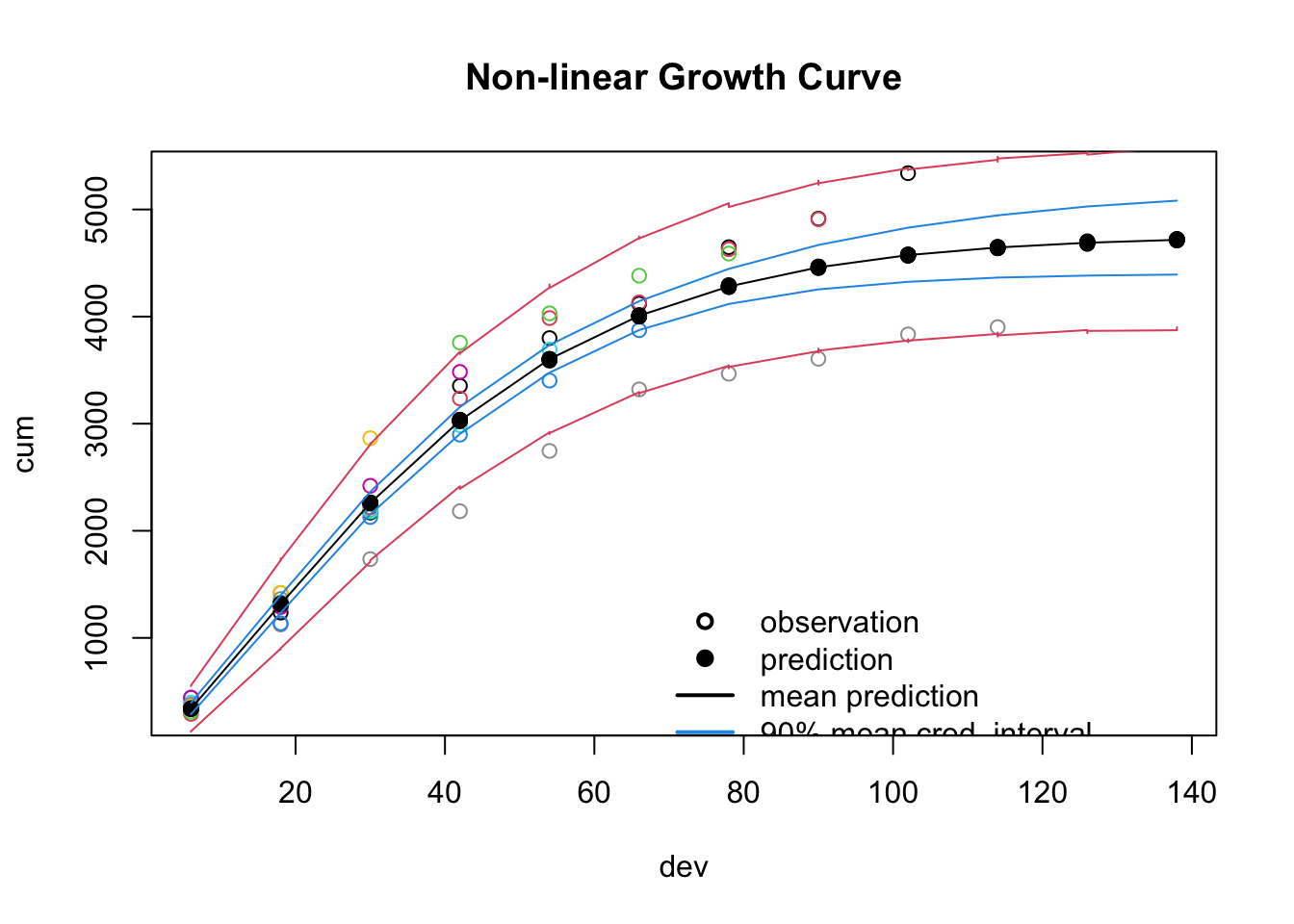

The 90% prediction credible interval captures most of the data and although this model might not be suitable for reserving individual accident years, it could provide an initial starting point for further investigations. Additionally, thanks to the Bayesian model I have access to the full distribution, not just point estimators and standard errors.

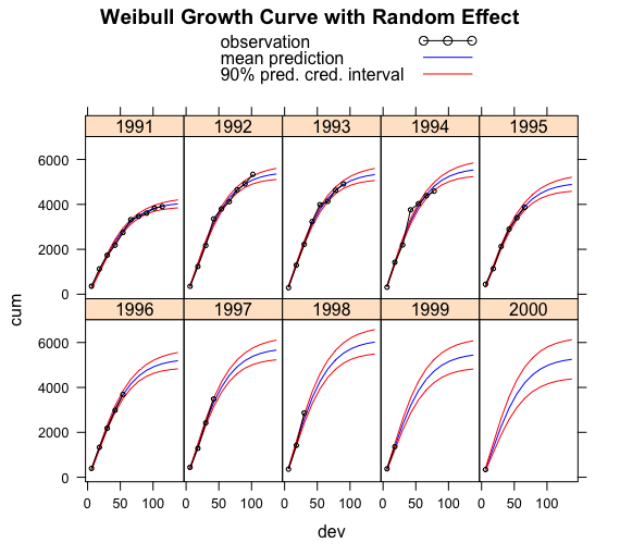
My next post will continue with this data set and the ideas of James Guszcza by allowing the ultimate loss cost to vary by accident year, treating it as a random effect. Here is a teaser of what the output will look like:

References

[1] David R. Clark. LDF Curve-Fitting and Stochastic Reserving: A Maximum Likelihood Approach. Casualty Actuarial Society, 2003. CAS Fall Forum.

[2] Guszcza, J. Hierarchical Growth Curve Models for Loss Reserving, 2008, CAS Fall Forum, pp. 146–173.

Session Info

R version 3.2.2 (2015-08-14)
Platform: x86_64-apple-darwin13.4.0 (64-bit)
Running under: OS X 10.11.1 (El Capitan)

locale:
[1] en_GB.UTF-8/en_GB.UTF-8/en_GB.UTF-8/C/en_GB.UTF-8/en_GB.UTF-8

attached base packages:
[1] stats     graphics  grDevices utils     datasets  methods  
[7] base     

other attached packages:
[1] rstan_2.8.0    ggplot2_1.0.1     Rcpp_0.12.1      
[4] nlme_3.1-122   lattice_0.20-33   ChainLadder_0.2.3

loaded via a namespace (and not attached):
 [1] nloptr_1.0.4       plyr_1.8.3         tools_3.2.2       
 [4] digest_0.6.8       lme4_1.1-10        statmod_1.4.21    
 [7] gtable_0.1.2       mgcv_1.8-8         Matrix_1.2-2      
[10] parallel_3.2.2     biglm_0.9-1        SparseM_1.7       
[13] proto_0.3-10       gridExtra_2.0.0    coda_0.18-1       
[16] stringr_1.0.0      MatrixModels_0.4-1 stats4_3.2.2      
[19] lmtest_0.9-34      grid_3.2.2         nnet_7.3-11       
[22] inline_0.3.14      tweedie_2.2.1      cplm_0.7-4        
[25] minqa_1.2.4        reshape2_1.4.1     car_2.1-0         
[28] actuar_1.1-10      magrittr_1.5       codetools_0.2-14  
[31] scales_0.3.0       MASS_7.3-44        splines_3.2.2     
[34] systemfit_1.1-18   rsconnect_0.3.79   pbkrtest_0.4-2    
[37] colorspace_1.2-6   labeling_0.3       quantreg_5.19     
[40] sandwich_2.3-4     stringi_1.0-1      munsell_0.4.2     
[43] zoo_1.7-12