Non-linear growth curves with Stan

I suppose the go to tool for fitting non-linear models in R is nls of the stats package. In this post I will show an alternative approach with Stan/RStan, as illustrated in the example, Dugongs: “nonlinear growth curve”, that is part of Stan’s documentation.

The original example itself is taken from OpenBUGS. The data describes the length and age measurements for 27 captured dugongs (sea cows). Carlin and Gelfand (1991) model the data using a nonlinear growth curve with no inflection point and an asymptote as \(x_i\) tends to infinity:

\[ \begin{aligned} Y_i \sim \mathcal{N}(\mu_i, \sigma^2),\; i = 1,\dots,27\\ \mu_i = \alpha - \beta \lambda^{x_i},\; \alpha,\, \beta > 0;\, 0 < \lambda < 1 \end{aligned} \]
Fitting the curve with nls gives the following results:

dat <- list(
  "N" = 27,  
  "x" =
    c(1, 1.5, 1.5, 1.5, 2.5, 4, 5, 5, 7, 8, 8.5, 9, 9.5, 9.5, 10, 
      12, 12, 13, 13, 14.5, 15.5, 15.5, 16.5, 17, 22.5, 29, 31.5),
  "Y" =
    c(1.8, 1.85, 1.87, 1.77, 2.02, 2.27, 2.15, 2.26, 2.47, 2.19, 
      2.26, 2.4, 2.39, 2.41, 2.5, 2.32, 2.32, 2.43, 2.47, 2.56, 2.65, 
      2.47, 2.64, 2.56, 2.7, 2.72, 2.57))

nlm <- nls(Y ~ alpha - beta * lambda^x, data=dat,
           start=list(alpha=1, beta=1, lambda=0.9))
summary(nlm)

## 
## Formula: Y ~ alpha - beta * lambda^x
## 
## Parameters:
##        Estimate Std. Error t value Pr(>|t|)    
## alpha   2.65807    0.06151   43.21  < 2e-16 ***
## beta    0.96352    0.06968   13.83  6.3e-13 ***
## lambda  0.87146    0.02460   35.42  < 2e-16 ***
## ---
## Signif. codes:  0 '***' 0.001 '**' 0.01 '*' 0.05 '.' 0.1 ' ' 1
## 
## Residual standard error: 0.09525 on 24 degrees of freedom
## 
## Number of iterations to convergence: 6 
## Achieved convergence tolerance: 3.574e-06

Writing the model in Stan requires a few more lines, but gives me also the opportunity to generate output from the posterior distributions.

stanmodel <- "
data {
  int<lower=0> N; 
  real x[N]; 
  real Y[N]; 
} 
parameters {
  real alpha; 
  real beta;  
  real<lower=.5,upper= 1> lambda; // original gamma in the JAGS example  
  real<lower=0> tau; 
} 
transformed parameters {
  real sigma; 
  real m[N];
  for (i in 1:N) 
    m[i] = alpha - beta * pow(lambda, x[i]);
  sigma = 1 / sqrt(tau); 
} 
model {
  // priors
  alpha ~ normal(0.0, 1000); 
  beta ~ normal(0.0, 1000); 
  lambda ~ uniform(.5, 1); 
  tau ~ gamma(.0001, .0001); 
  // likelihood
  Y ~ normal(m, sigma);   
}
generated quantities{
  real Y_mean[N]; 
  real Y_pred[N]; 
  for(i in 1:N){
    // Posterior parameter distribution of the mean
    Y_mean[i] = alpha - beta * pow(lambda, x[i]);
    // Posterior predictive distribution
    Y_pred[i] = normal_rng(Y_mean[i], sigma);   
}
}
"
library(rstan)
rstan_options(auto_write = TRUE)
options(mc.cores = parallel::detectCores())
fit <- stan(model_code = stanmodel, 
            model_name = "GrowthCurve", 
            data = dat)
print(fit, c("alpha", "beta", "lambda", "sigma"))

## Inference for Stan model: GrowthCurve.
## 4 chains, each with iter=2000; warmup=1000; thin=1; 
## post-warmup draws per chain=1000, total post-warmup draws=4000.
## 
##        mean se_mean   sd 2.5%  25%  50%  75% 97.5% n_eff Rhat
## alpha  2.65       0 0.07 2.53 2.61 2.65 2.69  2.80  1199    1
## beta   0.97       0 0.07 0.83 0.92 0.97 1.02  1.12  1767    1
## lambda 0.86       0 0.03 0.78 0.85 0.87 0.88  0.91  1096    1
## sigma  0.10       0 0.02 0.07 0.09 0.10 0.11  0.13  1792    1
## 
## Samples were drawn using NUTS(diag_e) at Sun Aug 16 08:09:28 2020.
## For each parameter, n_eff is a crude measure of effective sample size,
## and Rhat is the potential scale reduction factor on split chains (at 
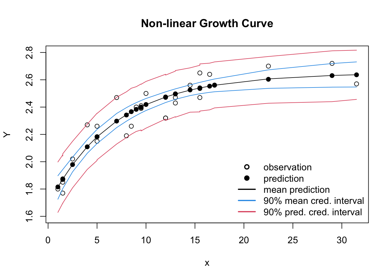
## convergence, Rhat=1).

The predicted parameters and errors are very much the same as in the least square output of nls, but with the Stan output I can also review the 90% credible intervals.

Y_mean <- extract(fit, "Y_mean")
Y_mean_cred <- apply(Y_mean$Y_mean, 2, quantile, c(0.05, 0.95))
Y_mean_mean <- apply(Y_mean$Y_mean, 2, mean)

Y_pred <- extract(fit, "Y_pred")
Y_pred_cred <- apply(Y_pred$Y_pred, 2, quantile, c(0.05, 0.95))
Y_pred_mean <- apply(Y_pred$Y_pred, 2, mean)

plot(dat$Y ~ dat$x, xlab="x", ylab="Y", 
     ylim=c(1.6, 2.8), main="Non-linear Growth Curve")
lines(dat$x, Y_mean_mean)
points(dat$x, Y_pred_mean, pch=19)
lines(dat$x, Y_mean_cred[1,], col=4)
lines(dat$x, Y_mean_cred[2,], col=4)
lines(dat$x, Y_pred_cred[1,], col=2)
lines(dat$x, Y_pred_cred[2,], col=2)
legend(x="bottomright", bty="n", lwd=2, lty=c(NA, NA, 1, 1,1),
       legend=c("observation", "prediction", "mean prediction",
                "90% mean cred. interval", "90% pred. cred. interval"),
       col=c(1,1,1,4,2),  pch=c(1, 19, NA, NA, NA))

Session Info

R version 3.2.2 (2015-08-14)
Platform: x86_64-apple-darwin13.4.0 (64-bit)
Running under: OS X 10.11.1 (El Capitan)

locale:
[1] en_GB.UTF-8/en_GB.UTF-8/en_GB.UTF-8/C/en_GB.UTF-8/en_GB.UTF-8

attached base packages:
[1] stats     graphics  grDevices utils     datasets 
[6] methods   base     

other attached packages:
[1] rstan_2.8.0        ggplot2_1.0.1.9003 Rcpp_0.12.1       

loaded via a namespace (and not attached):
 [1] colorspace_1.2-6 scales_0.3.0     plyr_1.8.3      
 [4] parallel_3.2.2   tools_3.2.2      inline_0.3.14   
 [7] gtable_0.1.2     gridExtra_2.0.0  codetools_0.2-14
[10] grid_3.2.2       stats4_3.2.2     munsell_0.4.2