Bayesian regression models using Stan in R

It seems the summer is coming to end in London, so I shall take a final look at my ice cream data that I have been playing around with to predict sales statistics based on temperature for the last couple of weeks [1], [2], [3].

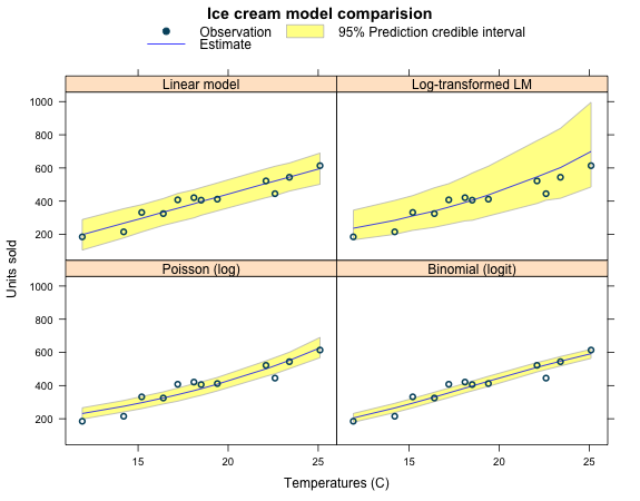
Here I will use the new brms (GitHub, CRAN) package by Paul-Christian Bürkner to derive the 95% prediction credible interval for the four models I introduced in my first post about generalised linear models. Additionally, I am interested to predict how much ice cream I should hold in stock for a hot day at 35ºC, such that I only run out of ice cream with a probability of 2.5%.

Stan models with brms

Like in my previous post about the log-transformed linear model with Stan, I will use Bayesian regression models to estimate the 95% prediction credible interval from the posterior predictive distribution.

Thanks to brms this will take less than a minute of coding, because brm allows me to specify my models in the usual formula syntax and I can leave it to the package functions to create and execute the Stan files.

Let’s start. Here is the data again: My models are written down in very much the same way as with glm. Only the binomial model requires a slightly different syntax. Here I use the default priors and link functions: Last week I wrote the Stan model for the log-transformed linear model myself. Here is the output of brm. The estimated parameters are quite similar, apart from \(\sigma\):

I access the underlying Stan model via log.lin.mod$model and note that the prior of \(\sigma\) is modelled via a Cauchy distribution, unlike the inverse Gamma I used last week. I believe that explains my small difference in \(\sigma\).

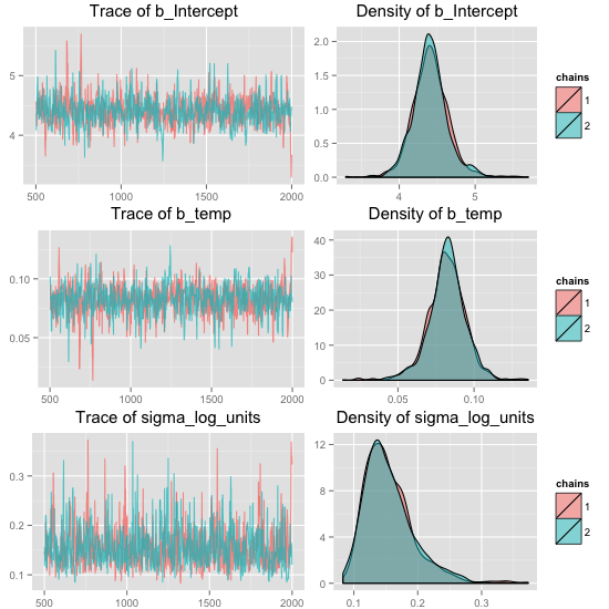
To review the model I start by plotting the trace and density plots for the MCMC samples.

Prediction credible interval

The predict function gives me access to the posterior predictive statistics, including the 95% prediction credible interval.

Combining the outputs of all four models into one data frame gives me then the opportunity to compare the prediction credible intervals of the four models in one chart. There are no big news in respect of the four models, but for the fact that here I can look at the posterior prediction credible intervals, rather then the theoretical distributions two weeks ago. The over-prediction of the log-transformed linear model is apparent again.

How much stock should I hold on a hot day?

Running out of stock on a hot summer’s day would be unfortunate, because those are days when sells will be highest. But how much stock should I hold?

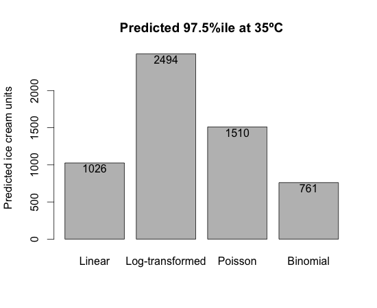
Well, if I set the probability of selling out at 2.5%, then I will have enough ice cream to sell with 97.5% certainty. To estimate those statistics I have to calculate the 97.5% percentile of the posterior predictive samples.

Ok, I have four models and four answers ranging from 761 to 2494. The highest number is more than 3 times the lowest number!

I had set the market size at 800 in my binomial model, so I am not surprised by its answer of 761. Also, I noted earlier that the log-normal distribution is skewed to the right, so that explains the high prediction of 2494. The Poisson model, like the log-transform linear model, has the implicit exponential growth assumption. Its mean forecast is well over 1000 as I pointed out earlier and hence the 97.5% prediction of 1510 is to be expected.

Conclusions

How much ice cream should I hold in stock? Well, if I believe strongly in my assumption of a market size of 800, then I should stick with the output of the binomial model, or perhaps hold 800 just in case.

Another aspect to consider would be the cost of holding unsold stock. Ice cream can usually be stored for some time, but the situation would be quite different for freshly baked bread or bunches of flowers that have to be sold quickly.

Session Info

Note, I used the developer version of brms from GitHub.

R version 3.2.2 (2015-08-14)
Platform: x86_64-apple-darwin13.4.0 (64-bit)
Running under: OS X 10.10.5 (Yosemite)

locale:
[1] en_GB.UTF-8/en_GB.UTF-8/en_GB.UTF-8/C/en_GB.UTF-8/en_GB.UTF-8

attached base packages:
[1] stats     graphics  grDevices utils     datasets 
[6] methods   base     

other attached packages:
[1] lattice_0.20-33 brms_0.4.1.9000 ggplot2_1.0.1  
[4] rstan_2.7.0-1   inline_0.3.14   Rcpp_0.12.0    

loaded via a namespace (and not attached):
 [1] codetools_0.2-14 digest_0.6.8     MASS_7.3-43     
 [4] grid_3.2.2       plyr_1.8.3       gtable_0.1.2    
 [7] stats4_3.2.2     magrittr_1.5     scales_0.2.5    
[10] stringi_0.5-5    reshape2_1.4.1   proto_0.3-10    
[13] tools_3.2.2      stringr_1.0.0    munsell_0.4.2   
[16] parallel_3.2.2   colorspace_1.2-6