Generalised Linear Models in R
Linear models are the bread and butter of statistics, but there is a lot more to it than taking a ruler and drawing a line through a couple of points.
Some time ago Rasmus Bååth published an insightful blog article about how such models could be described from a distribution centric point of view, instead of the classic error terms convention.
I think the distribution centric view makes generalised linear models (GLM) much easier to understand as well. That’s the purpose of this post.
Using data on ice cream sells statistics I will set out to illustrate different models, starting with traditional linear least square regression, moving on to a linear model, a log-transformed linear model and then on to generalised linear models, namely a Poisson (log) GLM and Binomial (logistic) GLM.
Along the way I aim to reveal the intuition behind a GLM and using Ramus’ distribution centric description. I hope to clarify why one would want to use different distributions and link functions.
The data
Here is the example data set I will be using. It shows units of ice cream sold at different temperatures. As expected more ice cream is sold at higher temperature.
library(arm) # for 'display' function only
icecream <- data.frame(
# http://www.statcrunch.com/5.0/viewreport.php?reportid=34965&groupid=1848
  temp=c(11.9, 14.2, 15.2, 16.4, 17.2, 18.1,
         18.5, 19.4, 22.1, 22.6, 23.4, 25.1),
  units=c(185L, 215L, 332L, 325L, 408L, 421L,
          406L, 412L, 522L, 445L, 544L, 614L)
  )
basicPlot <- function(...){
  plot(units ~ temp, data=icecream, bty="n", lwd=2,
       main="Ice cream units sold", col="#00526D",
       xlab="Temperatur (Celsius)",
       ylab="Units sold", ...)
  axis(side = 1, col="grey")
  axis(side = 2, col="grey")
}
basicPlot()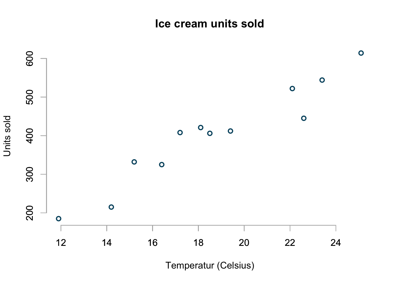
The challenge
I would like to create a model that predicts the units sold for any temperature, even outside the range of available data.
I am particular interested how my models will behave in the more extreme cases when it is freezing outside, say the temperature dropped to 0ºC and the prediction for a very hot summer’s day at 35ºC.
Linear least square
My first approach is to take a ruler and draw a straight line through the points, such that it minimises the average distance between the points and the line. That’s a basically a linear least square regression line:
basicPlot()
lsq.mod <- lsfit(icecream$temp, icecream$units)
abline(lsq.mod, col="orange", lwd=2)
legend(x="topleft", bty="n", lwd=c(2,2), lty=c(NA,1),
       legend=c("observation", "linear least square"),
         col=c("#00526D","orange"),  pch=c(1,NA))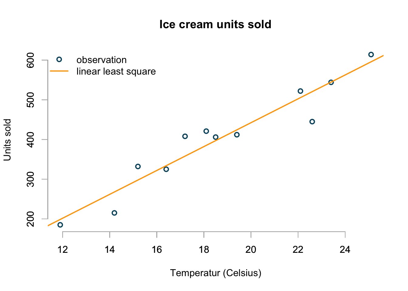
That’s easy and looks not unreasonable.
Linear regression
I believe the observation \(y_i\) was drawn from a Normal (aka Gaussian) distribution with a mean \(\mu_i\), depending on the temperature \(x_i\) and a constant variance \(\sigma^2\) across all temperatures.
On another day with the same temperature I might have sold a different quantity of ice cream, but over many days with the same temperature the average units of sold ice cream would converge towards \(\mu_i\).
Thus, using a distribution centric notation my model looks like this: \[ \begin{aligned} y_i & \sim \mathcal{N}(\mu_i, \sigma^2), \\ \mathbb{E}[y_i] & =\mu_i = \alpha + \beta x_i \; \text{for all}\; i \end{aligned} \] Note, going forward I will drop the \(\text{for all}\; i\) statement for brevity.
Or, alternatively I might argue that the residuals, the difference between the observations and predicted values, follow a Gaussian distribution with a mean of 0 and variance \(\sigma^2\): \[ \varepsilon_i = y_i - \mu_i \sim \mathcal{N}(0, \sigma^2) \] Furthermore, the equation \[ \mathbb{E}[y_i]=\mu_i = \alpha + \beta x_i \] states my believe that the expected value of \(y_i\) is identical to the parameter \(\mu_i\) of the underlying distribution, while the variance is constant.
The same model written in the classic error terms convention looks like this: \[ \begin{aligned} y_i & = \alpha + \beta x_i + \varepsilon_i\\ \varepsilon_i & \sim \mathcal{N}(0, \sigma^2) \end{aligned} \]
I think the probability distribution centric convention makes it clearer that my observation is just one realisation from a distribution. Furthermore, it emphasises that the parameter of the distribution is modelled linearly.
To model this in R explicitly I use the glm function, specifying the response distribution as Gaussian and the link function from the expected value of the distribution to its parameter as identity. And this is really the trick with a GLMs, it describes the distribution of the observations and how its expected value, often after a smooth transformation, relates to the actual measurements (predictors) in a linear way. The ‘link’ is the inverse function of the original transformation of the data.
That’s all its says on the GLM tin and that all there is.
lin.mod <- glm(units ~ temp, data=icecream,
              family=gaussian(link="identity"))
display(lin.mod)
## glm(formula = units ~ temp, family = gaussian(link = "identity"),
## data = icecream)
## coef.est coef.se
## (Intercept) -159.47 54.64
## temp 30.09 2.87
## ---
## n = 12, k = 2
## residual deviance = 14536.3, null deviance = 174754.9 (difference = 160218.6)
## overdispersion parameter = 1453.6
## residual sd is sqrt(overdispersion) = 38.13\[ \begin{aligned} y_i & \sim \mathcal{N}(\mu_i, \sigma^2)\\ \mu_i & = -159.5 + 30.1 x_i, \; \sigma & = 38.1 \end{aligned} \]
Although the linear model looks fine in the range of temperature observed, it doesn’t make much sense at 0ºC.
The intercept is at -159, which would mean that customers return on average 159 units of ice cream on a freezing day. Well, I don’t think so.
Log-transformed linear regression
Ok, perhaps I can transform the data first. Ideally I would like ensure that the transformed data has only positive values. The first transformation that comes to my mind in those cases is the logarithm.
So, let’s model the ice cream sales on a logarithmic scale. Thus my model changes to: \[ \begin{aligned} \log(y_i) & \sim \mathcal{N}(\mu_i, \sigma^2)\\ \mathbb{E}[\log(y_i)] & =\mu_i = \alpha + \beta x_i \end{aligned} \]
This model implies that I believe the sales follow a log-normal distribution, \(y_i \sim \log\mathcal{N}(\mu_i, \sigma^2)\), which means that I regard higher sales figures as more likely than lower sales figures, as the log-normal distribution is skewed to the right.
Although the model is still linear on a log-scale, I have to remember to transform the predictions back to the original scale (remember \(\mathbb{E}[\log(y_i)] \neq \log(\mathbb{E}[y_i])\)):
\[ \begin{aligned} y_i & \sim \log\mathcal{N}(\mu_i, \sigma^2)\\ \mathbb{E}[y_i] & = \exp(\mu_i + \sigma^2/2) \end{aligned} \]
log.lin.mod <- glm(log(units) ~ temp, data=icecream,
              family=gaussian(link="identity"))
display(log.lin.mod)
## glm(formula = log(units) ~ temp, family = gaussian(link = "identity"),
## data = icecream)
## coef.est coef.se
## (Intercept) 4.40 0.20
## temp 0.08 0.01
## ---
## n = 12, k = 2
## residual deviance = 0.2, null deviance = 1.4 (difference = 1.2)
## overdispersion parameter = 0.0
## residual sd is sqrt(overdispersion) = 0.14log.lin.sig <- summary(log.lin.mod)$dispersion
log.lin.pred <- exp(predict(log.lin.mod) + 0.5 * log.lin.sig)
basicPlot()
lines(icecream$temp, log.lin.pred, col="red", lwd=2)
legend(x="topleft", bty="n", lwd=c(2,2), lty=c(NA,1),
legend=c("observation", "log-transformed LM"),
col=c("#00526D","red"), pch=c(1,NA))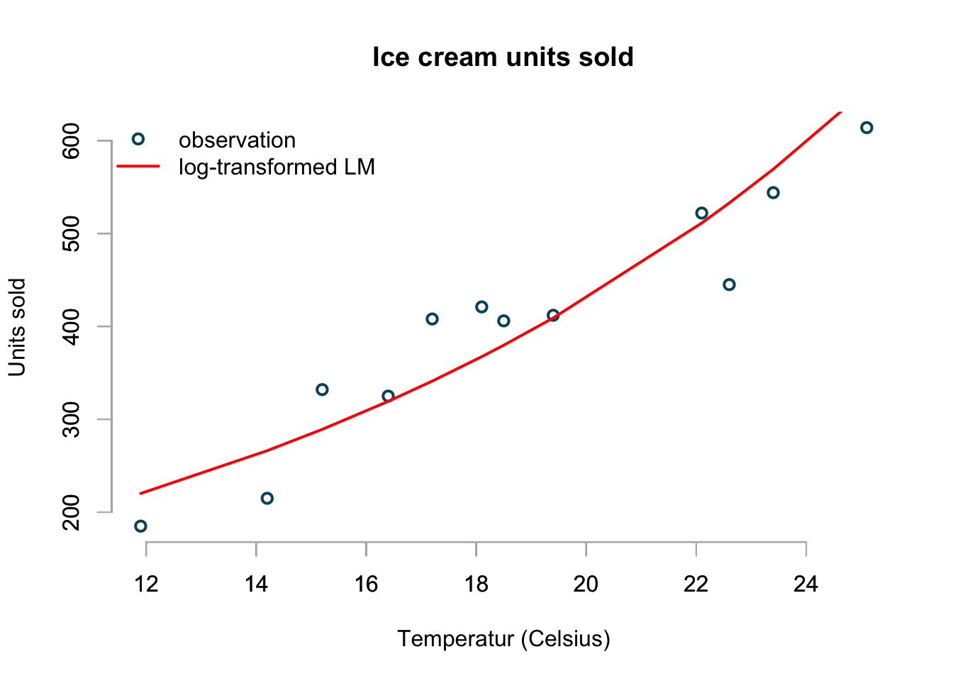
The plot looks a little better than the previous linear model and it predicts that I would sell on average 82 ice creams at a 0ºC:
exp(coef(log.lin.mod)[1])## (Intercept)
## 81.62131Although this model makes a little more sense, it appears that is over-predicts sells at lower and higher temperatures.
Furthermore, there is another problem with this model and the previous linear model as well.
The assumed model distributions generate real numbers, but my sales statistics are units and hence always whole numbers. Although the average number of units sold is likely to be a real number any draw from the model distribution should be a whole number.
Poisson regression
The classic approach for count data is the Poisson distribution.
The Poisson distribution has only one parameter, here \(\mu_i\), which is also its expected value. The canonical link function for \(\mu_i\) is the logarithm, which means I have to apply the exponential function to the linear model to get back to the original scale. Here is my model:
\[ \begin{aligned} y_i & \sim \text{Poisson}(\mu_i)\\ \log(\mu_i) & = \alpha + \beta x_i\\ \mathbb{E}[y_i] & =\exp(\alpha + \beta x_i) \end{aligned} \]
Let me say this again, although the expected value of my observation is a real number, the Poisson distribution will generate only whole numbers, in line with the actual sales.
pois.mod <- glm(units ~ temp, data=icecream,
              family=poisson(link="log"))
display(pois.mod)
## glm(formula = units ~ temp, family = poisson(link = "log"), data = icecream)
## coef.est coef.se
## (Intercept) 4.54 0.08
## temp 0.08 0.00
## ---
## n = 12, k = 2
## residual deviance = 60.0, null deviance = 460.1 (difference = 400.1)pois.pred <- predict(pois.mod, type="response")
basicPlot()
lines(icecream$temp, pois.pred, col="blue", lwd=2)
legend(x="topleft", bty="n", lwd=c(2,2), lty=c(NA,1),
legend=c("observation", "Poisson (log) GLM"),
col=c("#00526D","blue"), pch=c(1,NA))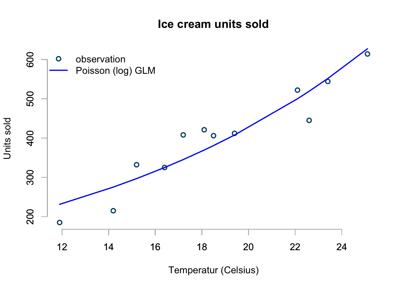
This looks pretty good. The interpretation of the coefficient should be clear
now. I have to use the exp function to make prediction of sales
for a given temperature. However, R will do this for me automatically, if I set in the
predict statement above type="response".
From the coefficients I can read off that a 0ºC I am expected to sell \(\exp(4.45)=94\) ice creams and that with each one degree increase in temperature the sales are predicted to increase by \(\exp(0.076) - 1 = 7.9\%\).
Note, the exponential function turns the additive scale into a multiplicative one.
So far, so good. My model is in line with my observations. Additionally, it will not predict negative sales and if I would simulate from a Poisson distribution with a mean given by the above model I will always only get whole numbers back.
However, my model will also predict that I should expect to sell over 1000 ice creams if temperature reach 32 Celsius:
predict(pois.mod, newdata=data.frame(temp=32), type="response")## 1
## 1056.651Perhaps the exponential growth in my model looks a little too good to be true. Indeed, I am pretty sure that my market will be saturated at around 800.
Binomial regression
Ok, let’s me think about the problem this way: I have 800 potential sales and I’d like to understand the proportion sold for a given temperature.
This suggests a binomial distribution for the number of successful sales out of 800. The key parameter for the binomial distribution is the probability of success, the probability that someone will buy my ice cream as a function of temperature.
Dividing my sales statistics by 800 would give me a first proxy for the probability of selling all ice cream.
Therefore I need an S-shape curve that maps the sales statistics into probabilities between 0 and 100%.
A canonical choice is the logistic function:
\[\text{logistic}(u) = logit^{-1}(u) = \frac{e^u}{e^u + 1} = \frac{1}{1 + e^{-u}}\]
With that my model can be described as:
\[ \begin{aligned} p_i & \sim \text{B}(n, \mu_i)\\ \mu_i & = \text{logit}^{-1}(\alpha + \beta x_i)\\ \mathbb{E}[p_i] & =\text{logit}(\alpha + \beta x_i) \end{aligned} \]
market.size <- 1000
icecream$opportunity <- market.size - icecream$units
bin.glm <- glm(cbind(units, opportunity) ~ temp, data=icecream,
    family=binomial(link = "logit"))
display(bin.glm)
## glm(formula = cbind(units, opportunity) ~ temp, family = binomial(link = "logit"),
## data = icecream)
## coef.est coef.se
## (Intercept) -2.85 0.10
## temp 0.13 0.01
## ---
## n = 12, k = 2
## residual deviance = 75.0, null deviance = 754.1 (difference = 679.1)bin.pred <- predict(bin.glm, type="response")*market.size
basicPlot()
lines(icecream$temp, bin.pred, col="purple", lwd=2)
legend(x="topleft", bty="n", lwd=c(2,2), lty=c(NA,1),
legend=c("observation", "Binomial (logit) GLM"),
col=c("#00526D","purple"), pch=c(1,NA))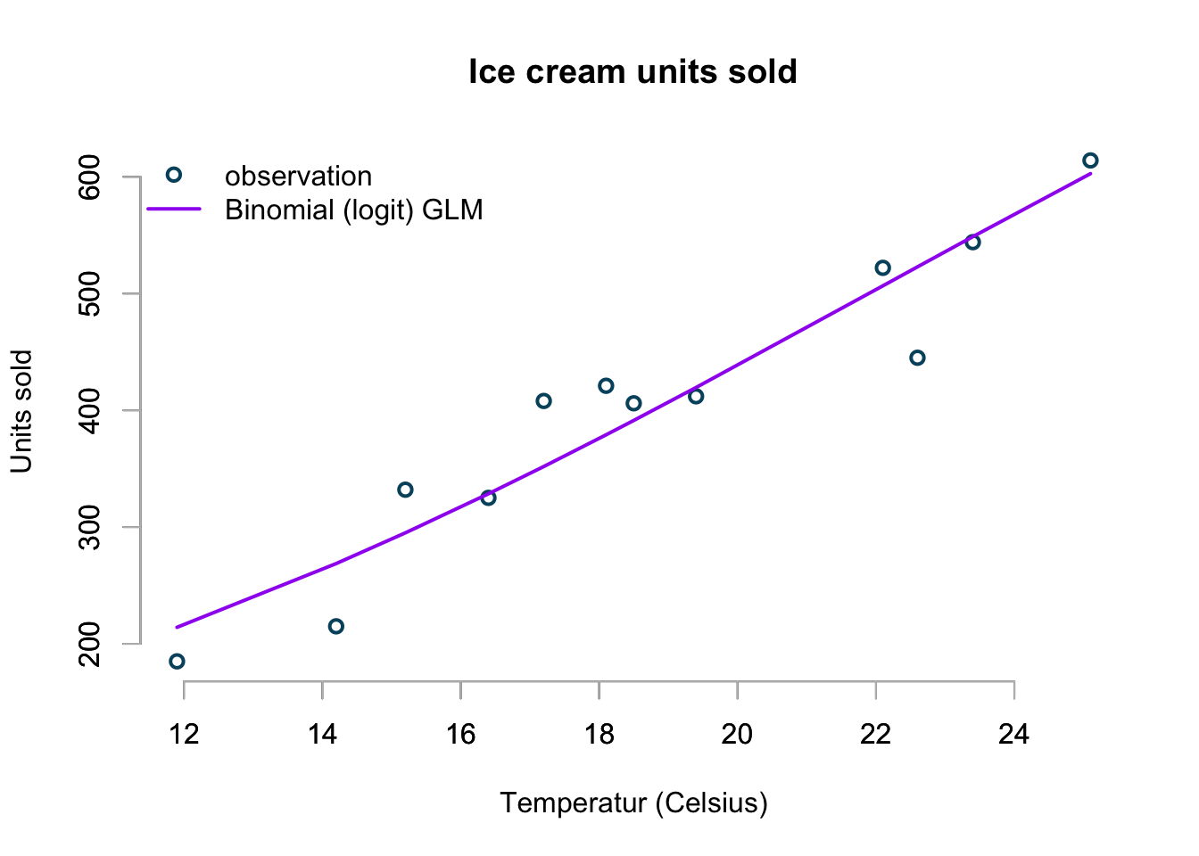
The chart doesn’t look too bad at all!
As the temperature rises higher and higher this model will predict that sales will reach market saturation, while all the other models so far would predict higher and higher sales.
I can predict the sales at 0ºC and 35ºC using the inverse of the logistic function, which is given in R as plogis:
# Sales at 0 Celsius
plogis(coef(bin.glm)[1])*market.size
## (Intercept)
## 54.78799# Sales at 35 Celsius
plogis(coef(bin.glm)[1] + coef(bin.glm)[2]*35)*market.size## (Intercept)
## 846.0892Summary
Let’s bring all the models together into one graph, with temperature ranging from 0 to 35ºC.
temp <- 0:35
p.lm <- predict(lin.mod, data.frame(temp=temp), type="response")
p.log.lm <- exp(predict(log.lin.mod, data.frame(temp=0:35), type="response") +
                  0.5 * summary(log.lin.mod)$dispersion)
p.pois <- predict(pois.mod, data.frame(temp=temp), type="response")
p.bin <- predict(bin.glm, data.frame(temp=temp), type="response")*market.size
basicPlot(xlim=range(temp), ylim=c(-20,market.size))
lines(temp, p.lm, type="l", col="orange", lwd=2)
lines(temp, p.log.lm, type="l", col="red", lwd=2)
lines(temp, p.pois, type="l", col="blue", lwd=2)
lines(temp, p.bin, type="l", col="purple", lwd=2)
legend(x="topleft",
       legend=c("observation",
                "linear model",
                "log-transformed LM",
                "Poisson (log) GLM",
                "Binomial (logit) GLM"),
       col=c("#00526D","orange", "red",
             "blue", "purple"),
       bty="n", lwd=rep(2,5),
       lty=c(NA,rep(1,4)),
       pch=c(1,rep(NA,4)))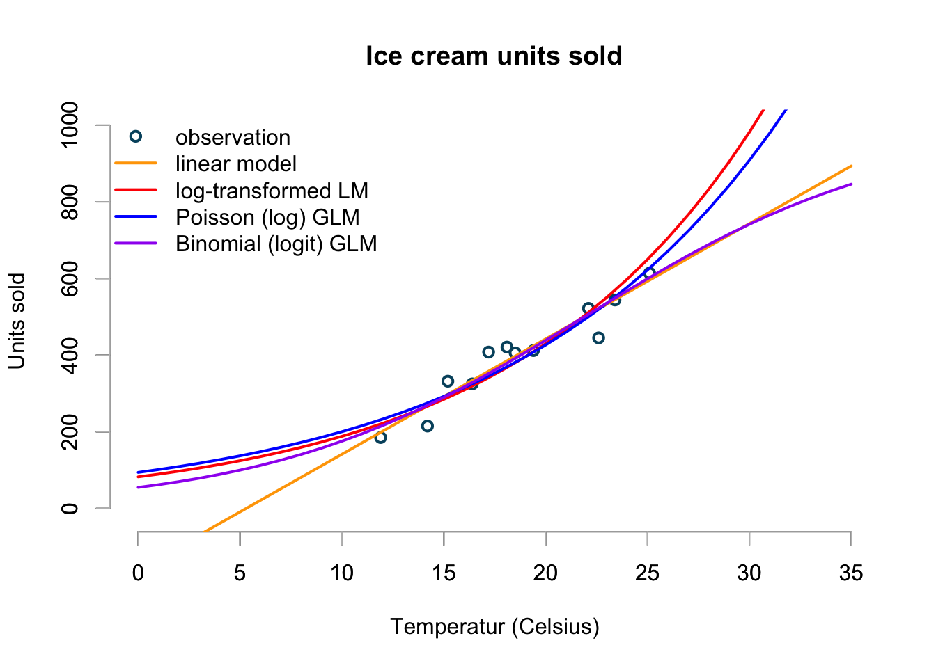
The chart shows the predictions of my four models over a temperature range from 0ºC to 35ºC. Although the linear model looks OK between 10ºC and perhaps 30ºC, it shows clearly its limitation. The log-transformed linear and Poisson models appear to give similar predictions, but will predict an ever accelerating increase in sales as temperature rise. I don’t believe this makes sense as even the most ice cream loving person can only eat so much ice cream on a really hot day. And that’s why I would go with the Binomial model to predict my ice cream sales.
Simulations
Having used the distribution centric view to describe my models leads naturally to simulations. If the models are good, then I shouldn’t be able to identify the real data from the simulation.
In all my models the linear structure was
\[g(\mu_i) = \alpha + \beta x_i\]
or in matrix notation
\[g(\mu_i) = A v\]
with \(A_{i,\cdot} = [1, x_i]\) and \(v=[\alpha, \beta]\), whereby \(A\) is the model matrix and \(v\) the vector of coefficients.
With that being said, let’s simulate data from each distribution for the temperatures measured in the original data and compare against the actual sales units.
n <- nrow(icecream)
A <- model.matrix(units ~ temp, data=icecream)
set.seed(1234)
(rand.normal <- rnorm(n,
                     mean = A %*% coef(lin.mod),
                     sd = sqrt(summary(lin.mod)$dispersion)))
## [1] 152.5502 278.3509 339.2073 244.5335 374.3981 404.4103 375.2385 403.3892
## [9] 483.9470 486.5775 526.3881 557.6662(rand.logtrans <- rlnorm(n,
meanlog = A %*% coef(log.lin.mod),
sdlog = sqrt(summary(log.lin.mod)$dispersion)))## [1] 196.0646 266.1002 326.8102 311.5621 315.0249 321.1920 335.3733 564.6961
## [9] 515.9348 493.4822 530.8356 691.2354(rand.pois <- rpois(n,
lambda = exp(A %*% coef(pois.mod))))## [1] 220 266 279 337 364 434 349 432 517 520 516 663(rand.bin <- rbinom(n,
size = market.size,
prob = plogis(A %*% coef(bin.glm))))## [1] 206 252 303 309 332 381 380 432 517 540 543 607basicPlot(ylim=c(100,700))
cols <- adjustcolor(c("orange", "red", "blue", "purple"),
alpha.f = 0.75)
points(icecream$temp, rand.normal, pch=19, col=cols[1])
points(icecream$temp, rand.logtrans, pch=19, col=cols[2])
points(icecream$temp, rand.pois, pch=19, col=cols[3])
points(icecream$temp, rand.bin, pch=19, col=cols[4])
legend(x="topleft",
legend=c("observation",
"linear model",
"log-transformed LM",
"Poisson (log) GLM",
"Binomial (logit) GLM"),
col=c("#00526D",cols),
lty=NA,
bty="n", lwd=rep(2,5),
pch=c(1,rep(19,4)))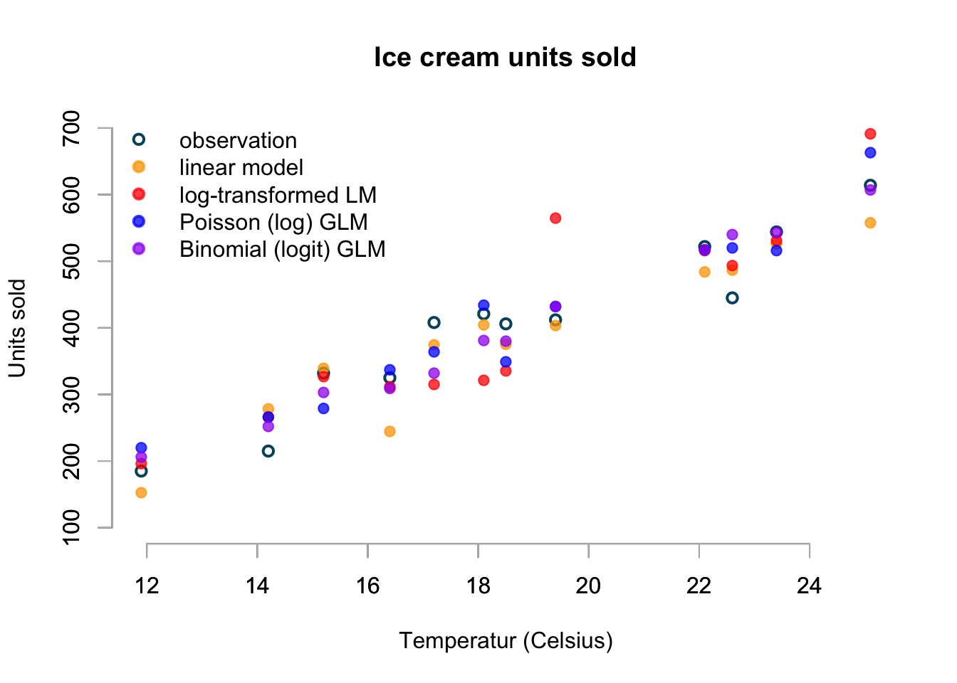
The chart displays just one simulation from each model, but I believe it shows already some interesting aspects. Not only do I see that the Poisson and Binomial model generate whole numbers, while the Gaussian and log-transformed Gaussian predict real numbers, I notice the skewness of the log-normal distribution in the red point as 19.4ºC.
Furthermore, the linear model predicts equally likely figures above and below the mean and at 16.4ºC the prediction appears a little low - perhaps as a result.
Additionally the high sales prediction at 25.1ºC of the log-transformed and Poisson model shouldn’t come as a surprise either.
Again, the simulation of the binomial model seems the most realistic to me.
Conclusions
I hope this little article illustrated the intuition behind generalised linear models.
Fitting a model to data requires more than just applying an algorithm. In particular it is worth to think about:
- the range of expected values: are they bounded or range from \(-\infty\) to \(\infty\)?
- the type of observations: do I expect real numbers, whole numbers or proportions?
- how to link the distribution parameters to the observations
Session Info
sessionInfo()## R version 4.1.0 (2021-05-18)
## Platform: aarch64-apple-darwin20 (64-bit)
## Running under: macOS Big Sur 11.5.1
##
## Matrix products: default
## BLAS: /Library/Frameworks/R.framework/Versions/4.1-arm64/Resources/lib/libRblas.dylib
## LAPACK: /Library/Frameworks/R.framework/Versions/4.1-arm64/Resources/lib/libRlapack.dylib
##
## locale:
## [1] en_US.UTF-8/en_US.UTF-8/en_US.UTF-8/C/en_US.UTF-8/en_US.UTF-8
##
## attached base packages:
## [1] stats graphics grDevices utils datasets methods base
##
## other attached packages:
## [1] arm_1.11-2 lme4_1.1-27.1 Matrix_1.3-4 MASS_7.3-54
##
## loaded via a namespace (and not attached):
## [1] Rcpp_1.0.7 lattice_0.20-44 png_0.1-7
## [4] assertthat_0.2.1 digest_0.6.27 utf8_1.2.2
## [7] R6_2.5.0 backports_1.2.1 evaluate_0.14
## [10] coda_0.19-4 highr_0.9 ggplot2_3.3.5
## [13] blogdown_1.4 pillar_1.6.1 rlang_0.4.11
## [16] minqa_1.2.4 rstudioapi_0.13 data.table_1.14.0
## [19] nloptr_1.2.2.2 jquerylib_0.1.4 rpart_4.1-15
## [22] checkmate_2.0.0 rmarkdown_2.9 splines_4.1.0
## [25] stringr_1.4.0 foreign_0.8-81 htmlwidgets_1.5.3
## [28] munsell_0.5.0 compiler_4.1.0 xfun_0.24
## [31] pkgconfig_2.0.3 base64enc_0.1-3 htmltools_0.5.1.1
## [34] nnet_7.3-16 tidyselect_1.1.1 tibble_3.1.3
## [37] gridExtra_2.3 htmlTable_2.2.1 bookdown_0.22
## [40] Hmisc_4.5-0 fansi_0.5.0 crayon_1.4.1
## [43] dplyr_1.0.7 grid_4.1.0 nlme_3.1-152
## [46] jsonlite_1.7.2 gtable_0.3.0 lifecycle_1.0.0
## [49] DBI_1.1.1 magrittr_2.0.1 scales_1.1.1
## [52] stringi_1.7.3 latticeExtra_0.6-29 bslib_0.2.5.1
## [55] ellipsis_0.3.2 generics_0.1.0 vctrs_0.3.8
## [58] boot_1.3-28 Formula_1.2-4 RColorBrewer_1.1-2
## [61] tools_4.1.0 glue_1.4.2 purrr_0.3.4
## [64] jpeg_0.1-9 abind_1.4-5 survival_3.2-11
## [67] yaml_2.2.1 colorspace_2.0-2 cluster_2.1.2
## [70] knitr_1.33 sass_0.4.0Citation
For attribution, please cite this work as:Markus Gesmann (Aug 04, 2015) Generalised Linear Models in R. Retrieved from https://magesblog.com/post/2015-08-04-generalised-linear-models-in-r/
@misc{ 2015-generalised-linear-models-in-r,
author = { Markus Gesmann },
title = { Generalised Linear Models in R },
url = { https://magesblog.com/post/2015-08-04-generalised-linear-models-in-r/ },
year = { 2015 }
updated = { Aug 04, 2015 }
}