Posterior predictive output with Stan

I continue my Stan experiments with another insurance example. Here I am particular interested in the posterior predictive distribution from only three data points. Or, to put it differently I have a customer of three years and I’d like to predict the expected claims cost for the next year to set or adjust the premium.

The example is taken from section 16.17 in Loss Models: From Data to Decisions [1]. Some time ago I used the same example to get my head around a Bayesian credibility model.

Suppose the claims likelihood distribution is believed to follow an exponential distribution for a given parameter \(\Theta\). The prior parameter distribution on \(\Theta\) is assumed to be a gamma distribution with parameters \(\alpha=4, \beta=1000\): \[ \begin{aligned}\Theta & \sim \mbox{Gamma}(\alpha, \beta)\\ \ell_i & \sim \mbox{Exp}(\Theta) , \; \forall i \in N \end{aligned} \] In this case the predictive distribution is a Pareto II distribution with density \(f(x) = \frac{\alpha \beta^\alpha}{(x+\beta)^{\alpha+1}}\) and a mean of \(\frac{\beta}{\alpha-1} = 333.33\).

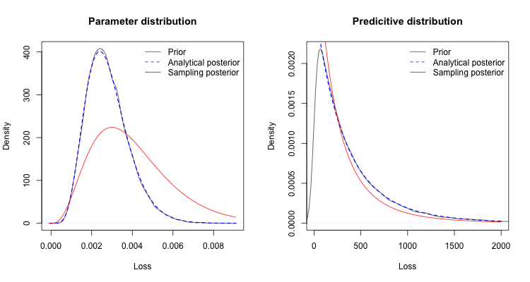
I have three independent observations, namely losses 100, 950 and 450. The posterior predictive expected loss is 416.67 and can be derived analytical, as shown in my earlier post. Now let me reproduce the answer with Stan as well.

Implementing the model in Stan is straightforward and I follow the same steps as in my simple example of last week. However, here I am also interested in the posterior predictive distribution, hence I add a generated quantities code block.

The output shows a simulated predictive mean of 416.86, close to the analytical answer. I can also read out that the 75%ile of the posterior predictive distribution is a loss of 542 vs. 414 from the prior predictive. That means every four years I shouldn’t be surprised to observe a loss in excess of 500. Further I note that 90% of losses are expected to be less than 950, or in other words the observation in my data may reflect the outcome of an event with a 1 in 10 return period.

Comparing the sampling output from Stan with the analytical output gives me some confidence that I am doing the ‘right thing’.

References

[1] Klugman, S. A., Panjer, H. H. & Willmot, G. E. (2004), Loss Models: From Data to Decisions, Wiley Series in Probability and Statistics.

Session Info

R version 3.2.0 (2015-04-16)
Platform: x86_64-apple-darwin13.4.0 (64-bit)
Running under: OS X 10.10.3 (Yosemite)

locale:
[1] en_GB.UTF-8/en_GB.UTF-8/en_GB.UTF-8/C/en_GB.UTF-8/en_GB.UTF-8

attached base packages:
[1] stats graphics grDevices utils datasets methods base     

other attached packages:
[1] lattice_0.20-31 actuar_1.1-8 rstan_2.6.0 inline_0.3.14  
[5] Rcpp_0.11.6    

loaded via a namespace (and not attached):
[1] tools_3.2.0  codetools_0.2-11 grid_3.2.0 stats4_3.2.0