Kalman filter example visualised with R

Motivation

Suppose I have a little robot that moves autonomously over my desk. How would the robot know where it is? Well, suppose the robot can calculate from its wheels’ movements how far it went and an additional sensor (e.g. GPS-like) provides also information about its location. Of course both pieces of information will be imprecise. How can the various signals be combined?

This is a classic scenario for the Kalman filter. Its key assumptions are that the errors/noise are Gaussian and that the state space evolution \(x_t\) from one time step to the next is linear, so is the mapping to the sensor signals \(y_t\). For the example I will use it reads:

\[ \begin{aligned} x_{t+1} & = A x_t + w,\quad w \sim N(0,Q)\\ y_t &=G x_t + \nu, \quad \nu \sim N(0,R)\\ x_0 & \sim N(\hat{x}_0, \Sigma_0) \end{aligned} \]

With \(A, Q, G, R, \Sigma_0\) matrices of appropriate dimensions. The Kalman filter provides recursive estimators for the expected position \(\hat{x}_{t+1}\):

\[ \begin{aligned} \hat{x}_{t+1} &= A \hat{x}_t + K_{t} (y_t - G \hat{x}_t) \\ K_{t} &= A \Sigma_t G' (G \Sigma_t G' + R)^{-1}\\ \Sigma_{t+1} &= A \Sigma_t A' - K_{t} G \Sigma_t A' + Q \end{aligned} \]

Start with a prior

Let’s say at time \(t_0\) the robot has the expected position \(\hat{x}_0 = (0.2, -0.2)\). That means, the robot doesn’t know its location on the table with certainty. Further I shall assume that the probability density function of the position follows a Normal distribution with covariance matrix \(\Sigma_0 = \left[\begin{array}{cc}0.4 & 0.3\\0.3 & 0.45\end{array}\right]\).

The prior distribution of the robot’s position can be visualised in R with a contour plot.

library(mnormt)
xhat <- c(0.2, -0.2)
Sigma <- matrix(c(0.4, 0.3, 
                  0.3, 0.45), ncol=2)
x1 <- seq(-2, 4,length=151)
x2 <- seq(-4, 2,length=151)
f <- function(x1,x2, mean=xhat, varcov=Sigma) 
  dmnorm(cbind(x1,x2), mean,varcov)
z <- outer(x1,x2, f)
mycols <- topo.colors(100,0.5)
image(x1,x2,z, col=mycols, main="Prior density",
      xlab=expression('x'[1]), ylab=expression('x'[2]))
contour(x1,x2,z, add=TRUE)
points(0.2, -0.2, pch=19)
text(0.1, -0.2, labels = expression(hat(x)), adj = 1)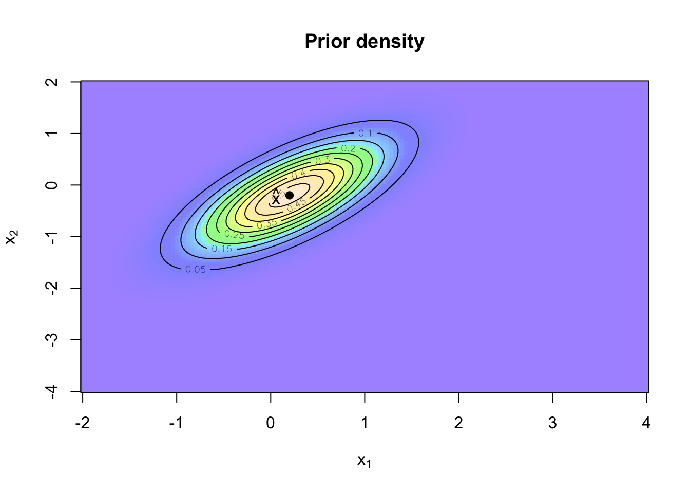

Sensor information

The ‘GPS’ sensor provides also data about the location of the robot, again the sensor signal can be regarded as the expected position with some noise. Suppose the reading of the sensor is \(y_0=(2.3, -1.9)\). I will assume that the sensor signal has an error following a Normal distribution, with a covariance matrix \(R=0.5 \Sigma_0\).

Conceptually I think about it like this, given that the robot is at position \(x\), what would be the likelihood that the sensor reading is \(y\,|\,x\,\)? The Kalman filter assumes a linear mapping from \(x\) to \(y\):

\[ \begin{aligned} y & = G x + \nu \mbox{ with } \nu \sim N(0,R) \end{aligned} \] In my case \(G\) will be the identity matrix. Let’s add the sensor information to the plot.

R <- 0.5 * Sigma
z2 <- outer(x1,x2, f, mean=c(2.3, -1.9), varcov=R)
image(x1, x2, z2, col=mycols, main="Sensor density")
contour(x1, x2, z2, add=TRUE)
points(2.3, -1.9, pch=19)
text(2.2, -1.9, labels = "y", adj = 1)
contour(x1, x2,z, add=TRUE)
points(0.2, -0.2, pch=19)
text(0.1, -0.2, labels = expression(hat(x)), adj = 1)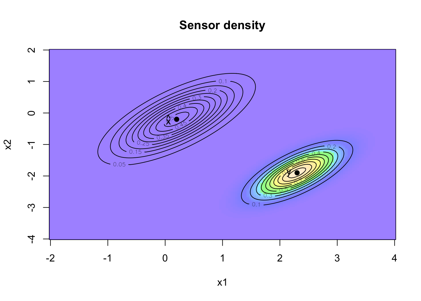

Filtering

I have two pieces of information about the location of the robot, both with a Normal distribution, my prior is \(x \sim N(\hat{x}, \Sigma)\) and for the distribution of my sensor I have \(y\,|\,x \sim N(Gx, R)\).

What I would like to know is the location of the robot given the sensor reading:

\[ \begin{aligned} p(x \,|\, y) & = \frac{p(y \,|\, x) \, p(x)} {p(y)} \end{aligned} \] Now, because \(x, y\) are Normal and \(G\) is the identity matrix, I know that the posterior distribution of \(x \,|\, y\) is Normal again, with parameters (see conjugate prior):

\[ \begin{aligned} \hat{x}_f & = (\Sigma^{-1} + R^{-1})^{-1} (\Sigma^{-1} \hat{x} + R^{-1} y) \\ \Sigma_f & = (\Sigma^{-1} + R^{-1})^{-1} \end{aligned} \] Using the matrix inversion identity

\[ \begin{aligned} (A^{-1} + B^{-1})^{-1} & = A - A (A + B)^{-1}A = A (A + B)^{-1} B \end{aligned} \]

I can write the above as:

\[ \begin{aligned} \hat{x}_f & = (\Sigma - \Sigma (\Sigma + R)^{-1}\Sigma)(\Sigma^{-1} \hat{x} + R^{-1}y)\\ & =\hat{x} - \Sigma (\Sigma + R)^{-1} \hat{x} + \Sigma R^{-1} y -\Sigma (\Sigma + R)^{-1}\Sigma R^{-1}y\\ & = \hat{x} + \Sigma (\Sigma + R)^{-1} (y - \hat{x})\\ & = (1.667, -1.333)\\ \Sigma_f &= \Sigma - \Sigma (\Sigma + R)^{-1} \Sigma\\ &=\left[\begin{array}{lll} 0.133 & 0.10\\ 0.100 & 0.15 \end{array} \right] \end{aligned} \]

In the more general case when \(G\) is not the identity matrix I have

\[ \begin{aligned} \hat{x}_f & = \hat{x} + \Sigma G' (G \Sigma G' + R)^{-1} (y - G \hat{x})\\ \Sigma_f &= \Sigma - \Sigma G' (G \Sigma G' + R)^{-1} G \Sigma \end{aligned} \]

The updated posterior probability density function \(p(x\,|\,y)=N(\hat{x}_f, \Sigma_f)\) is visualised in the chart below.

G <- diag(2)
y <- c(2.4, -1.9)
xhatf <- xhat + Sigma %*% t(G) %*% solve(G %*% Sigma %*% t(G) + R) %*% (y - G %*% xhat)
Sigmaf <- Sigma - Sigma %*% t(G) %*% solve(G %*% Sigma %*% t(G) + R) %*% G %*% Sigma
z3 <- outer(x1, x2, f, mean=c(xhatf), varcov=Sigmaf)
image(x1, x2, z3, col=mycols,
      xlab=expression('x'[1]), ylab=expression('x'[2]),
      main="Filtered density")
contour(x1, x2, z3, add=TRUE)
points(xhatf[1], xhatf[2], pch=19)
text(xhatf[1]-0.1, xhatf[2],
     labels = expression(hat(x)[f]), adj = 1)
lb <- adjustcolor("black", alpha=0.5)
contour(x1, x2, z, add=TRUE, col=lb)
points(0.2, -0.2, pch=19, col=lb)
text(0.1, -0.2, labels = expression(hat(x)), adj = 1, col=lb)
contour(x1, x2, z2, add=TRUE, col=lb)
points(2.3, -1.9, pch=19, col=lb)
text(2.2, -1.9,labels = "y", adj = 1, col=lb)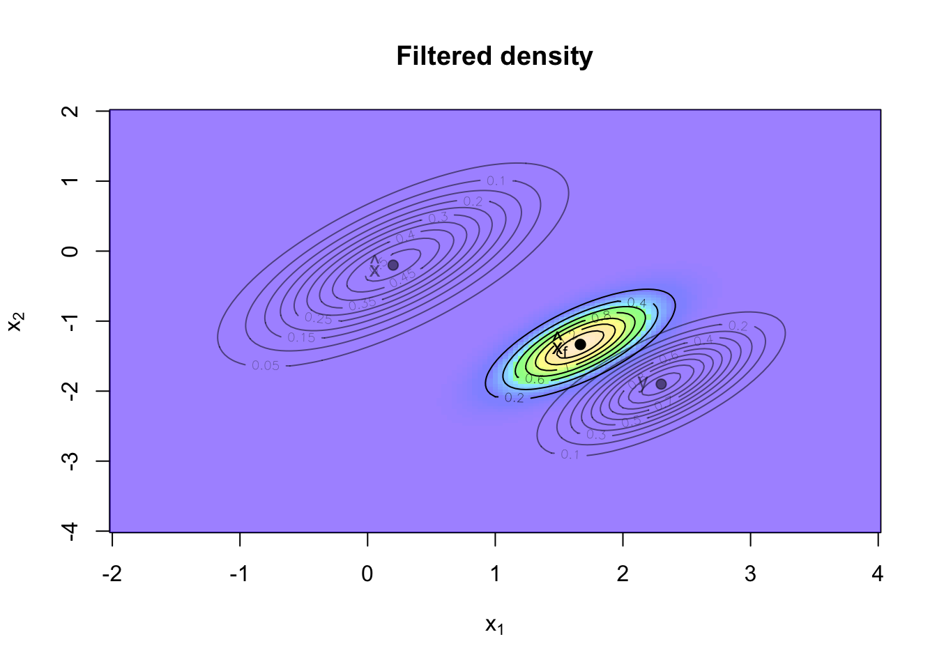

I can see how the prior and likelihood distributions have influenced the posterior distribution of the robot’s location. The sensor information is regarded more credible than the prior information and hence the posterior is closer to the sensor data.

Forecasting

Ok, I have a better understanding of the robot’s position at time \(t_0\), but the robot is moving and what I’d like to know is where it will be after one time step.

Suppose I have a linear model that explains how the state evolves over time, e.g. based on wheel spin. Again, I will assume a Gaussian process. In this toy example I follow the assumptions of Sargent and Stachurski, although this doesn’t make much sense for the robot:

\[ \begin{aligned} x_{t+1} & = A x_t + w_{t+1} \mbox{, where } w_t \sim N(0, Q) \end{aligned} \]

with

\[ \begin{split} A = \left( \begin{array}{cc} 1.2 & 0.0 \\ 0.0 & -0.2 \end{array} \right), \qquad Q = 0.3 \Sigma \end{split} \]

As all the processes are linear and Normal the calculations are straightforward:

\[ \begin{aligned} \mathbf{E} [A x_f + w] &= A \, \mathbf{E} [x_f] + \mathbf{E} [w]\\ &= A \hat{x}_f\\ &= A \hat{x} + A \Sigma G' (G \Sigma G' + R)^{-1}(y - G \hat x) \end{aligned} \]

\[ \begin{aligned} \operatorname{Var} [A x_f + w] & = A \operatorname{Var}[x_f] A' + Q\\ &= A \Sigma_f A' + Q\\ &= A \Sigma A' - A \Sigma G' (G \Sigma G' + R)^{-1} G \Sigma A' + Q \end{aligned} \]

The matrix \(A \Sigma G' (G \Sigma G' + R)^{-1}\) is often written as \(K\) and called the Kalman gain. Using this notation, I can summarise the results as follows:

\[ \begin{split} \begin{aligned} \hat{x}_{new} &:= A \hat{x} + K (y - G \hat{x}) \\ \Sigma_{new} &:= A \Sigma A' - K G \Sigma A' + Q \nonumber \end{aligned} \end{split} \]

Adding the prediction to my chart gives me:

A <- matrix(c(1.2, 0,
              0, -0.2), ncol=2)
Q <- 0.3 * Sigma
K <- A %*% Sigma %*% t(G) %*% solve(G%*% Sigma %*% t(G) + R)
xhatnew <- A %*% xhat + K %*% (y - G %*% xhat)
Sigmanew <- A %*% Sigma %*% t(A) - K %*% G %*% Sigma %*% t(A) + Q
z4 <- outer(x1,x2, f, mean=c(xhatnew), varcov=Sigmanew)
image(x1, x2, z4, col=mycols,
      xlab=expression('x'[1]), ylab=expression('x'[2]),
      main="Predictive density")
contour(x1, x2, z4, add=TRUE)
points(xhatnew[1], xhatnew[2], pch=19)
text(xhatnew[1]-0.1, xhatnew[2],
     labels = expression(hat(x)[new]), adj = 1)
contour(x1, x2, z3, add=TRUE, col=lb)
points(xhatf[1], xhatf[2], pch=19, col=lb)
text(xhatf[1]-0.1, xhatf[2], col=lb, 
     labels = expression(hat(x)[f]), adj = 1)
contour(x1, x2, z, add=TRUE, col=lb)
points(0.2, -0.2, pch=19, col=lb)
text(0.1, -0.2, labels = expression(hat(x)), adj = 1, col=lb)
contour(x1, x2, z2, add=TRUE, col=lb)
points(2.3, -1.9, pch=19, col=lb)
text(2.2, -1.9,labels = "y", adj = 1, col=lb)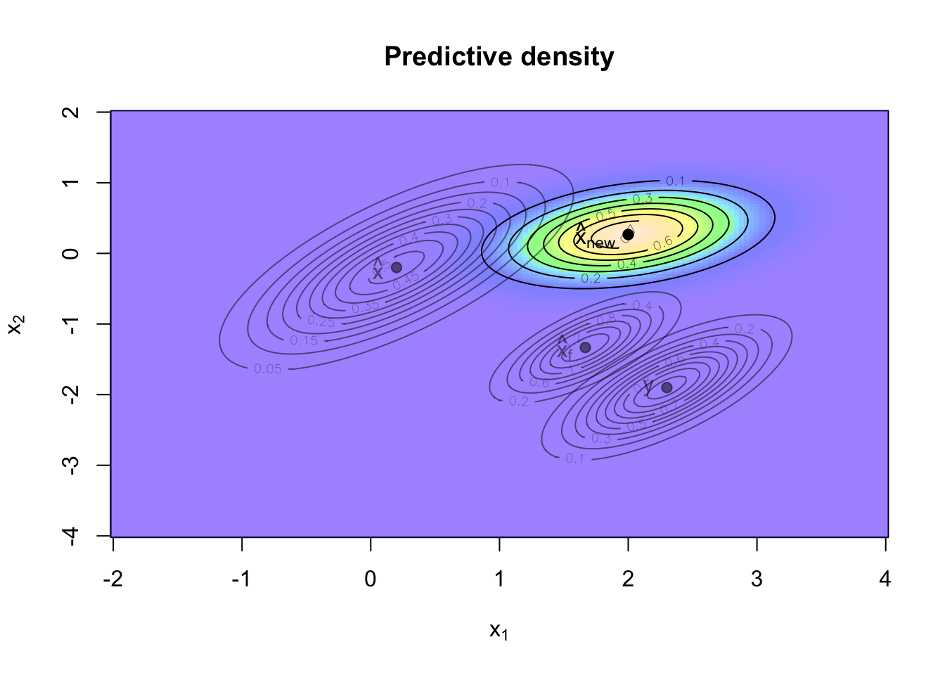

That’s it, having gone through the updating process for one time step gives me the recursive Kalman filter iteration mentioned above.

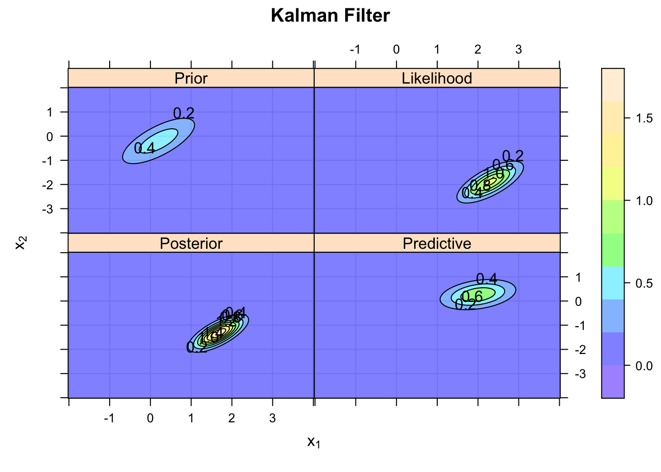
Another way to visualise the four steps can be achieved with the lattice package:

library(lattice)
grid <- expand.grid(x=x1,y=x2)
grid$Prior <- as.vector(z)
grid$Likelihood <- as.vector(z2)
grid$Posterior <- as.vector(z3)
grid$Predictive <- as.vector(z4)
contourplot(Prior + Likelihood + Posterior + Predictive ~ x*y, 
            data=grid, col.regions=mycols, region=TRUE,
            as.table=TRUE, 
            xlab=expression(x[1]),
            ylab=expression(x[2]),
            main="Kalman Filter",
            panel=function(x,y,...){
              panel.grid(h=-1, v=-1)
              panel.contourplot(x,y,...)
            })

Session Info

R version 3.1.2 (2014-10-31)
Platform: x86_64-apple-darwin13.4.0 (64-bit)

locale:
[1] en_GB.UTF-8/en_GB.UTF-8/en_GB.UTF-8/C/en_GB.UTF-8/en_GB.UTF-8

attached base packages:
[1] stats graphics grDevices utils datasets methods base     

other attached packages:
[1] lattice_0.20-29 mnormt_1.5-1   

loaded via a namespace (and not attached):
[1] grid_3.1.2  tools_3.1.2