Notes from the Kölner R meeting, 12 December 2014

Last week’s Cologne R user group meeting was the best attended so far, and it was a remarkable event - I believe not a single line of R code was shown. Still, it was an R user group meeting with two excellent talks, and you will understand shortly why not much R code needed to be displayed.

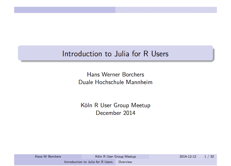
Introduction to Julia for R Users

Download slides

Hans Werner Borchers joined us from Mannheim to give an introduction to Julia for R users. Julia is a high-level, high-performance dynamic programming language for technical computing. The language has gained some considerable traction over the last two years and it was great to get an overview from a familiar perspective.

Interestingly, as Hans Werner pointed out, Julia is by far not the only new language around the block. Indeed, over the last decade nearly every year saw the announcement of a new language. Also big tech companies such as Microsoft, Google, Mozilla and Apple are trying to push their own programming languages: F# (2005), Go (2009), Rust (2010) and Swift (2014) respectively.

Over the more recent years we notice a movement towards the use of LLVM (Low Level Virtual Machine), on which Julia is based as well and which makes it fast. The just in time compilation demands a little mind shift if you come from R, where the mantra for speed is: vectorise - remove all for-loops. Well, the opposite is true for Julia, because your code will be compiled. For-loops are much easier to understand for the underlying compiler. Hans Werner’s slides provide some good examples to get you started and pointers to further resources.

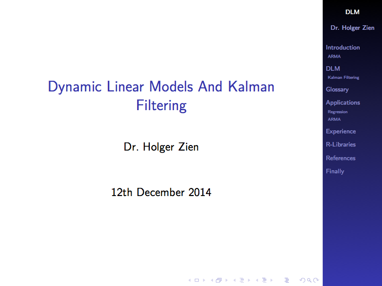
Dynamic Linear Models and Kalman Filtering

Download slides

Forecasting time series was the topic of Holger Zien’s talk. Holger gained his first experience with time series during his PhD, when he worked with experimental sensor data. That meant he had lots of data, which could often be regarded stationary as well.

Nowadays, his challenges can be very different, sometimes only a few data points from a non-stationary process are available, and yet he is still expected to predict the future.

Dynamic linear models (dlm) can provide a remedy in those situations. In their simplest version a dlm links system and observational equations in the following way:

\[ \begin{aligned} y_t & = F \theta_t + \nu_t\quad\mbox{observation eq. }\\ \theta_t & = G \theta_{t-1} + \omega_t\quad\mbox{system eq.} \end{aligned} \]

with \(\nu_t, \omega_t\) mutually independent random variables. A special case of dynamic linear models is the well known Kalman filter. In the more general case \(y_t\) and \(\theta_t\) are vectors and \(F_t, G_t\) are time variant matrices.

Holger explained that a dlm can principally be used for three purposes:

• Filtering: Estimate of the current value of the state/system variable.
• Smoothing: Estimate of past values of the state/system variable, i.e., estimating at time \(t\) given measurements up to time \(t' > t\).
• Forecasting: Forecasting future observations or values of the state/system variable.

With this introduction outlined Holger showed us how various ARMA and linear regression models can be expressed as dlm. His talk concluded with some remarks about his personal experience and references to various R packages, articles and books.

Next Kölner R meeting

The next meeting is scheduled for 6 March 2015.

Please get in touch if you would like to present and share your experience, or indeed if you have a request for a topic you would like to hear more about. For more details see also our Meetup page.

Thanks again to Bernd Weiß for hosting the event and Revolution Analytics for their sponsorship.