Not only verbs but also believes can be conjugated

Following on from last week, where I presented a simple example of a Bayesian network with discrete probabilities to predict the number of claims for a motor insurance customer, I will look at continuous probability distributions today. Here I follow example 16.17 in Loss Models: From Data to Decisions [1].

Suppose there is a class of risks that incurs random losses following an exponential distribution (density \(f(x) = \Theta {e}^{- \Theta x}\)) with mean \(1/\Theta\). Further, I believe that \(\Theta\) varies according to a gamma distribution (density $f(x)= x^{- 1} e^{- x } $) with shape \(\alpha=4\) and rate \(\beta=1000\).

In the same way as I had good and bad driver in my previous post, here I have clients with different characteristics, reflected by the gamma distribution.

The textbook tells me that the unconditional mixed distribution of an exponential distribution with parameter \(\Theta\), whereby \(\Theta\) has a gamma distribution, is a Pareto II distribution (density \(f(x) = \frac{\alpha \beta^\alpha}{(x+\beta)^{\alpha+1}}\)) with parameters \(\alpha,\, \beta\). Its k-th moment is given in the general case by

\[ E[X^k] = \frac{\beta^k\Gamma(k+1)\Gamma(\alpha - k)}{\Gamma(\alpha)},\; -1 < k < \alpha. \]

Thus, I can calculate the prior expected loss (\(k=1\)) as \(\frac{\beta}{\alpha-1}=\) 333.33.

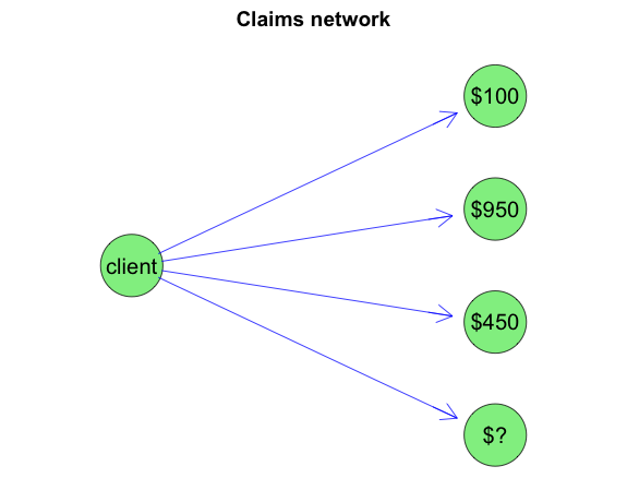
Now suppose I have three independent observations, namely losses of 100, 950 and 450 over the last 3 years. The mean loss is 500, which is higher than the 333.33 of my model.

Question: How should I update my belief about the client’s risk profile to predict the expected loss cost for year 4 given those 3 observations?

Visually I can regard this scenario as a graph, with evidence set for years 1 to 3 that I want to propagate through to year 4.

It turns out that in this case I can solve this problem analytically as the prior and posterior parameter distributions have a conjugate relationship. It means that the posterior parameter distribution is of the same distribution family as the prior, here a gamma, with updated posterior hyper-parameters.

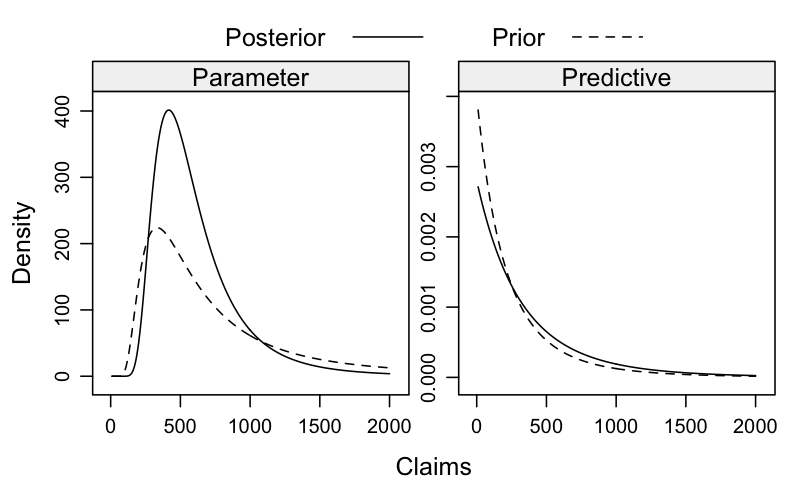
Skipping the maths, I have the following posterior hyper-parameters for my given data (\(n\)=number of data points, \(c\)=claims in year \(i\)) \[ (\alpha +n,\, \beta + \sum_i c_i) \]

The posterior predictive distribution is a Pareto II distribution as mentioned above, with the derived posterior hyper-parameters. I can calculate the posterior predictive expected claims amount as (1000+1500)/(4+3-1)=2500/(7-1)=416.67, which is higher than the prior 333.33, but still less than the actual average loss of 500.

Ok, let’s visualise this. The following chart shows the prior and posterior parameter and predictive distributions. It shows nicely how the distributions shift based on the observed data.

Note that I can calculate the posterior predictive expected loss from the parameters and data directly:

\[ \frac{\beta + \sum c_i}{\alpha + n - 1} = \frac{\alpha - 1}{\alpha+n-1}\frac{\beta}{\alpha-1} + \frac{n}{\alpha + n - 1}\bar{c} \]

That’s the weighted sum of the posterior predictive expected loss \(\mu:=\frac{\beta}{\alpha-1}\) and the sample mean \(\bar{c}\). And as the number of data points increases, the sample mean gains weight or in other words credibility.

Indeed, suppose I set \(Z_n:=\frac{n}{\alpha+n-1}\) then \((1-Z_n)=\frac{\alpha-1}{\alpha+n-1}\) and hence I can write my formula as

\[ (1-Z_n)\,\mu + Z_n \,\bar{c}, \]

with \(Z_n\) as my credibility factor.

References

[1] Klugman, S. A., Panjer, H. H. & Willmot, G. E. (2004), Loss Models: From Data to Decisions, Wiley Series in Probability and Statistics.

Session Info

R version 3.0.2 (2013-09-25)
Platform: x86_64-apple-darwin10.8.0 (64-bit)

locale:
[1] en_GB.UTF-8/en_GB.UTF-8/en_GB.UTF-8/C/en_GB.UTF-8/en_GB.UTF-8
 
attached base packages:
[1] grid      stats     graphics  grDevices utils     datasets  methods  
[8] base     
 
other attached packages:
[1] lattice_0.20-24 actuar_1.1-6    Rgraphviz_2.6.0 igraph_0.6.6   
[5] graph_1.40.0    knitr_1.5      
 
loaded via a namespace (and not attached):
[1] BiocGenerics_0.8.0 evaluate_0.5.1     formatR_0.10      
[4] parallel_3.0.2     stats4_3.0.2       stringr_0.6.2     
[7] tools_3.0.2