Predicting claims with a Bayesian network

Here is a little Bayesian Network to predict the claims for two different types of drivers over the next year, see also example 16.15 in [1].

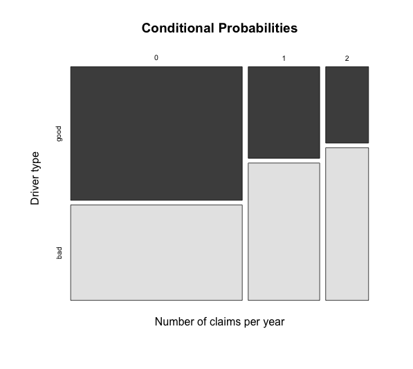
Let’s assume there are good and bad drivers. The probabilities that a good driver will have 0, 1 or 2 claims in any given year are set to 70%, 20% and 10%, while for bad drivers the probabilities are 50%, 30% and 20% respectively.

Further I assume that 75% of all drivers are good drivers and only 25% would be classified as bad drivers. Therefore the average number of claims per policyholder across the whole customer base would be:

0.75*(0*0.7 + 1*0.2 + 2*0.1) + 0.25*(0*0.5 + 1*0.3 + 2*0.2) = 0.475

Now a customer of two years asks for his renewal. Suppose he had no claims in the first year and one claim last year. How many claims should I predict for next year? Or in other words, how much credibility should I give him?

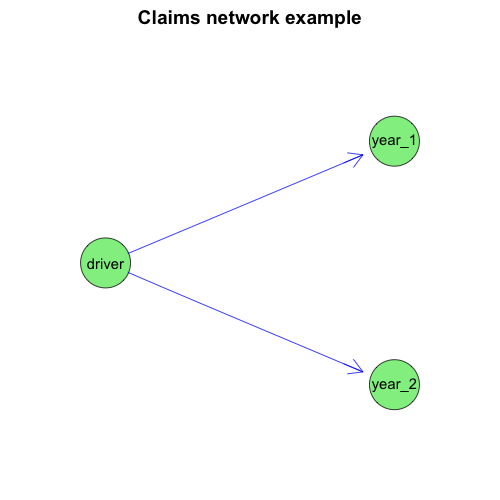
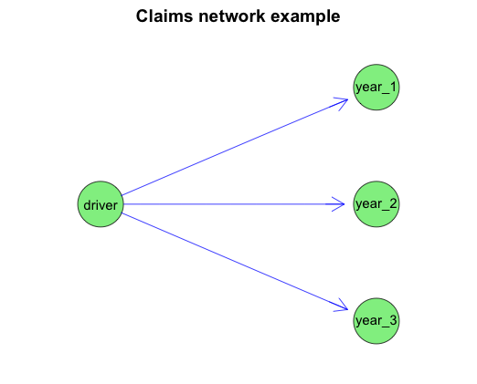
To answer the above question I present the data here as a Bayesian Network using the gRain package [2]. I start with the contingency probability tables for the driver type and the conditional probabilities for 0, 1 and 2 claims in year 1 and 2. As I assume independence between the years I set the same probabilities. I can now review my model as a mosaic plot (above) and as a graph (below) as well.

Next, I set the client’s evidence (0 claims in year one and 1 claim in year two) and propagate these back through my network to estimate the probabilities that the customer is either a good (73.68%) or a bad (26.32%) driver. Knowing that a good driver has on overage 0.4 claims a year and a bad driver 0.7 claims I predict the number of claims for my customer with the given claims history as 0.4789.

Alternatively I could have added a third node for year 3 and queried the network for the probabilities of 0, 1 or 2 claims given that the customer had zero claims in year 1 and one claim in year 2. The sum product of the number of claims and probabilities gives me again an expected claims number of 0.4789.

References

[1] Klugman, S. A., Panjer, H. H. & Willmot, G. E. (2004), Loss Models: From Data to Decisions, Wiley Series in Proability and Statistics.

[2] Søren Højsgaard (2012). Graphical Independence Networks with the gRain Package for R. Journal of Statistical Software, 46(10), 1-26. URL http://www.jstatsoft.org/v46/i10/

Session Info

R version 3.0.2 (2013-09-25)
Platform: x86_64-apple-darwin10.8.0 (64-bit)

locale:
[1] en_GB.UTF-8/en_GB.UTF-8/en_GB.UTF-8/C/en_GB.UTF-8/en_GB.UTF-8

attached base packages:
[1] grid      stats     graphics  grDevices utils     datasets  methods  
[8] base     

other attached packages:
[1] Rgraphviz_2.6.0 gRain_1.2-2     gRbase_1.6-12   graph_1.40.0   

loaded via a namespace (and not attached):
[1] BiocGenerics_0.8.0 igraph_0.6.6       lattice_0.20-24    Matrix_1.1-0      
[5] parallel_3.0.2     RBGL_1.38.0        stats4_3.0.2       tools_3.0.2