Minimise residual sum of squares

I start with an x-y data set, which I believe has a linear relationship and therefore I’d like to fit y against x by minimising the residual sum of squares.

dat=data.frame(x=c(1,2,3,4,5,6), 
               y=c(1,3,5,6,8,12))

Next, I create a function that calculates the residual sum of square of my data against a linear model with two parameter. Think of y = par[1] + par[2] * x.

min.RSS <- function(data, par) {
              with(data, sum((par[1] + par[2] * x - y)^2))
}

Optim minimises a function by varying its parameters. The first argument of optim are the parameters I’d like to vary, par in this case; the second argument is the function to be minimised, min.RSS. The tricky bit is to understand how to apply optim to your data. The solution is the ... argument in optim, which allows me to pass other arguments through to min.RSS, here my data. Therefore I can use the following statement:

(result <- optim(par = c(0, 1), fn = min.RSS, data = dat))

## $par
## [1] -1.266846  2.028620
## 
## $value
## [1] 2.819048
## 
## $counts
## function gradient 
##       89       NA 
## 
## $convergence
## [1] 0
## 
## $message
## NULL

Let me plot the result:

plot(y ~ x, data = dat, main="Least square regression")
abline(a = result$par[1], b = result$par[2], col = "red")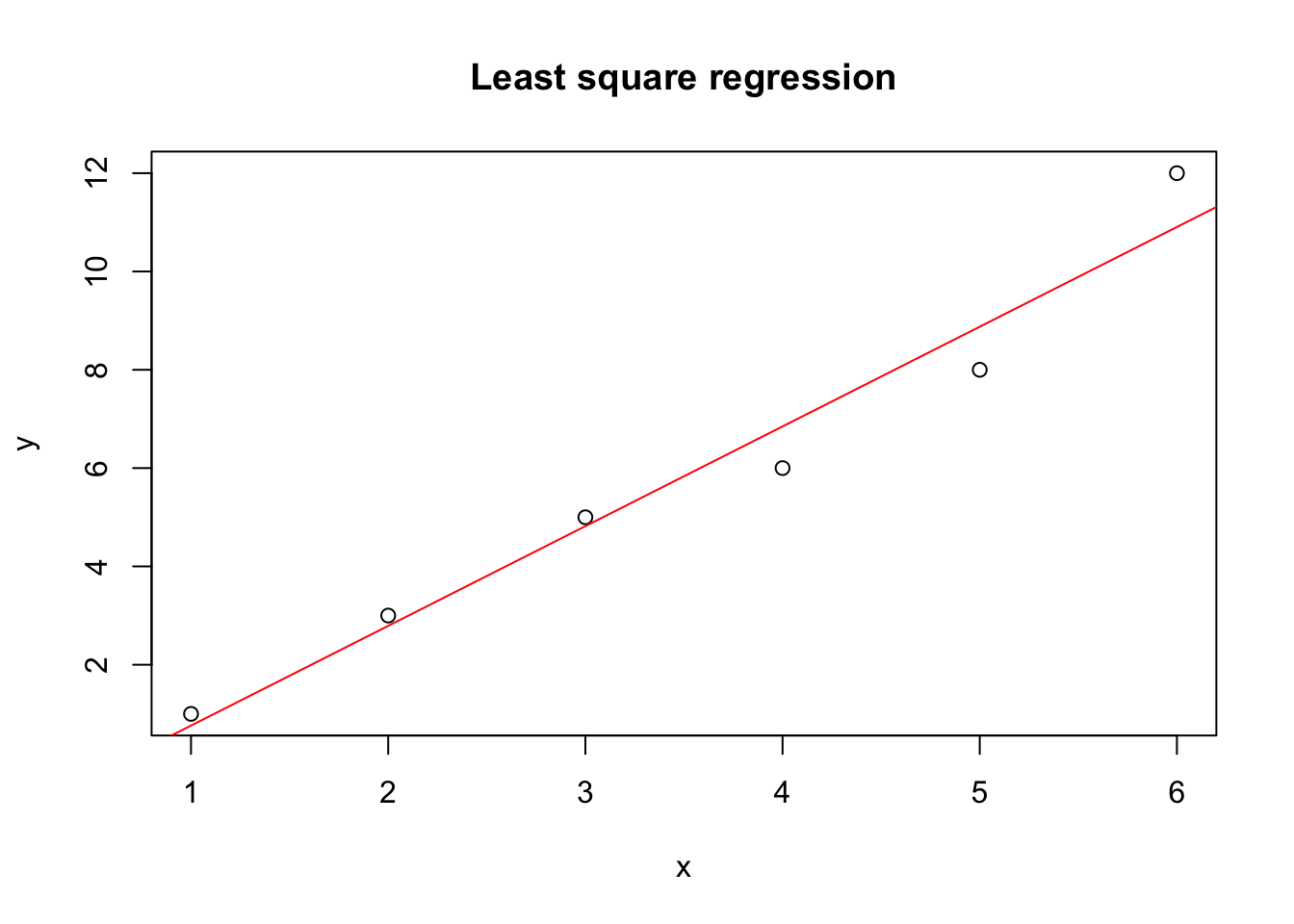

Great, this looks reasonable. How does it compare against the built in linear regression in R?

lm(y ~ x, data = dat)

## 
## Call:
## lm(formula = y ~ x, data = dat)
## 
## Coefficients:
## (Intercept)            x  
##      -1.267        2.029

Spot on! I get the same answer.

Maximum likelihood

In my second example I look at count data and I would like to fit a Poisson distribution to this data.

Here is my data:

obs = c(1, 2, 3, 4, 5, 6, 7, 8, 9, 10, 11, 12, 13, 17, 42, 43)
freq = c(1392, 1711, 914, 468, 306, 192, 96, 56, 35, 17, 15, 6, 2, 2, 1, 1)
x <- rep(obs, freq)
plot(table(x), main="Count data")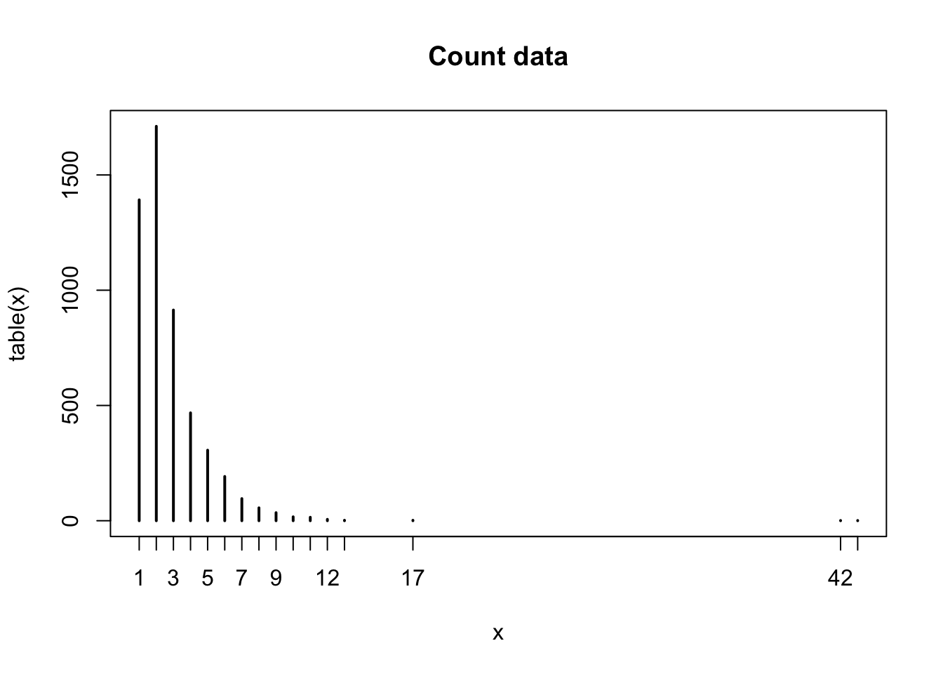

To fit a Poisson distribution to x I don’t minimise the residual sum of squares, instead I maximise the likelihood by varying its parameter \(\lambda\).

The likelihood function is given by:

lklh.poisson <- function(x, lambda) lambda^x/factorial(x) * exp(-lambda)

and the sum of the log-liklihood function is:

log.lklh.poisson <- function(x, lambda){ 
                     -sum(x * log(lambda) - log(factorial(x)) - lambda) 
                     }

By default optim searches for parameters, which minimise the function fn. In order to find a maximium, all I have to do is change the sign of the function, hence -sum(...).

optim(par = 2, log.lklh.poisson, x = x)

## Warning in optim(par = 2, log.lklh.poisson, x = x): one-dimensional optimization by Nelder-Mead is unreliable:
## use "Brent" or optimize() directly

## $par
## [1] 2.703516
## 
## $value
## [1] 9966.067
## 
## $counts
## function gradient 
##       24       NA 
## 
## $convergence
## [1] 0
## 
## $message
## NULL

Ok, the warning message tells me that I shoud use another optimisation algorithm, as I have a one dimensional problem - a single parameter. Thus, I follow the advise and get:

optim(par = 2, fn = log.lklh.poisson, x = x, method = "Brent", lower = 2, upper = 3)

## $par
## [1] 2.703682
## 
## $value
## [1] 9966.067
## 
## $counts
## function gradient 
##       NA       NA 
## 
## $convergence
## [1] 0
## 
## $message
## NULL

It’s actually the same result. Let’s compare the result to fitdistr, which uses maximum liklihood as well.

library(MASS)
fitdistr(x, "Poisson")

##      lambda  
##   2.70368239 
##  (0.02277154)

No surprise here, it gives back the mean, which is the maximum likelihood parameter.

mean(x)

## [1] 2.703682

For more information on optimisation and mathematical programming with R see the CRAN Task View on this subject.

Session Info

sessionInfo()

## R version 3.6.2 (2019-12-12)
## Platform: x86_64-apple-darwin15.6.0 (64-bit)
## Running under: macOS Catalina 10.15.3
## 
## Matrix products: default
## BLAS:   /Library/Frameworks/R.framework/Versions/3.6/Resources/lib/libRblas.0.dylib
## LAPACK: /Library/Frameworks/R.framework/Versions/3.6/Resources/lib/libRlapack.dylib
## 
## locale:
## [1] en_GB.UTF-8/en_GB.UTF-8/en_GB.UTF-8/C/en_GB.UTF-8/en_GB.UTF-8
## 
## attached base packages:
## [1] stats     graphics  grDevices utils     datasets  methods   base     
## 
## other attached packages:
## [1] MASS_7.3-51.5
## 
## loaded via a namespace (and not attached):
##  [1] compiler_3.6.2  magrittr_1.5    bookdown_0.17   tools_3.6.2    
##  [5] htmltools_0.4.0 yaml_2.2.0      Rcpp_1.0.3      stringi_1.4.5  
##  [9] rmarkdown_2.1   blogdown_0.17   knitr_1.27      stringr_1.4.0  
## [13] digest_0.6.23   xfun_0.12       rlang_0.4.4     evaluate_0.14