Reserving based on log-incremental payments in R, part III

This is the third post about Christofides’ paper on Regression models based on log-incremental payments [1]. The first post covered the fundamentals of Christofides’ reserving model in sections A - F, the second focused on a more realistic example and model reduction of sections G - K. Today’s post will wrap up the paper with sections L - M and discuss data normalisation and claims inflation.

I will use the same triangle of incremental claims data as introduced in my previous post. The final model had three parameters for origin periods and two parameters for development periods. It is possible to reduce the model further as Christofides illustrates in section L onwards by using an inflation index to bring all claims payments to current value and a claims volume adjustment or weight for each origin period to normalise the triangle.

In his example Christofides uses claims volume adjustments for the origin years and an earning or inflation index for the different payment calendar years. The claims volume adjustments aims to normalise the triangle for similar exposures across origin periods, while the earnings index, which measures largely wages and other forms of compensations, is used as a first proxy for claims inflation. Note that the earnings index shows significant year on year changes from 5% to 9%. Barnett and Zehnwirth [2] would probably recommend to add further parameters for the calendar year effects to the model.

# Page D5.36
ClaimsVolume <- data.frame(origin=0:6, 
                           volume.index=c(1.43, 1.45, 1.52, 1.35, 1.29, 1.47, 1.91))
# Page D5.36
EarningIndex <- data.frame(cal=0:6, 
                           earning.index=c(1.55, 1.41, 1.3, 1.23, 1.13, 1.05, 1))
# Year on year changes
round((1-EarningIndex$earning.index[-1]/EarningIndex$earning.index[-7]),2)

## [1] 0.09 0.08 0.05 0.08 0.07 0.05

# [1] 0.09 0.08 0.05 0.08 0.07 0.05

dat <- merge(merge(dat, ClaimsVolume), EarningIndex)

# Normalise data for volume and earnings
dat$logvalue.ind.inf <- with(dat, log(value/volume.index*earning.index))

with(dat, interaction.plot(dev, origin, logvalue.ind.inf))
points(1+dat$dev, dat$logvalue.ind.inf, pch=16, cex=0.8)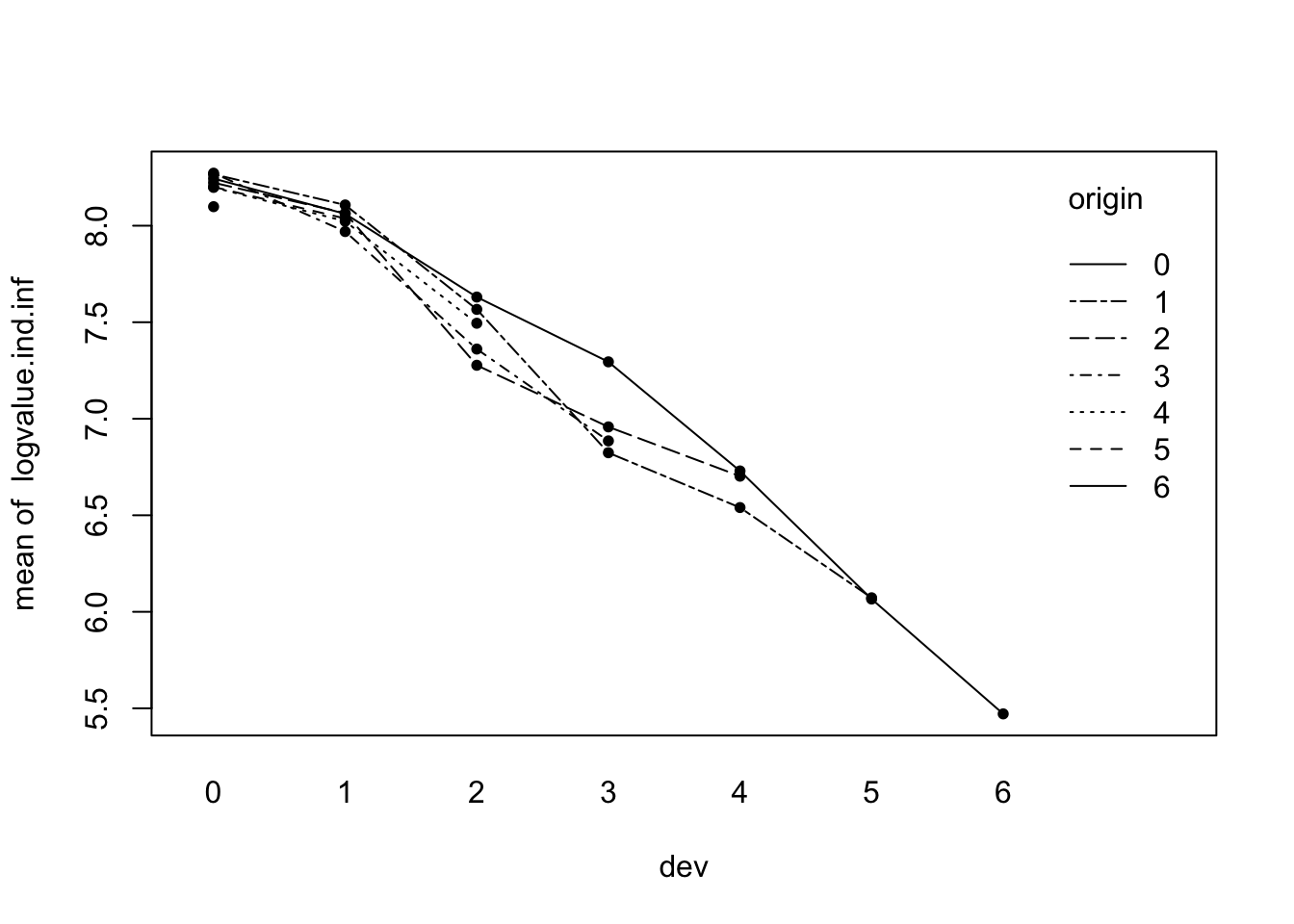

Indeed, the interaction plot shows the various origin years now to be much more closely grouped. Only the single point of the last origin period stands out now. Christofides tests several models with different numbers of origin levels, but I am happy with the minimal model using only one parameter for the origin period, namely the intercept:

# Page D5.39
summary(Fit4 <- lm(logvalue.ind.inf ~  d + s, data=na.omit(dat)))

## 
## Call:
## lm(formula = logvalue.ind.inf ~ d + s, data = na.omit(dat))
## 
## Residuals:
##      Min       1Q   Median       3Q      Max 
## -0.24591 -0.05066  0.01044  0.05202  0.26070 
## 
## Coefficients:
##             Estimate Std. Error t value Pr(>|t|)    
## (Intercept)  8.50073    0.05271 161.278  < 2e-16 ***
## d           -0.28598    0.06901  -4.144 0.000342 ***
## s           -0.48889    0.01725 -28.337  < 2e-16 ***
## ---
## Signif. codes:  0 '***' 0.001 '**' 0.01 '*' 0.05 '.' 0.1 ' ' 1
## 
## Residual standard error: 0.1179 on 25 degrees of freedom
## Multiple R-squared:  0.9795, Adjusted R-squared:  0.9779 
## F-statistic: 597.2 on 2 and 25 DF,  p-value: < 2.2e-16

All coefficients are significant and I am left with a model of only three parameters. The residual plots suggest that my model is reasonable, only the QQ-plot shows that the distribution of the residuals is a little bit skewed.

op <- par(mfrow=c(2,2), mar=c(4,4,2,2))
attach(model.frame(Fit4))
with(na.omit(dat), 
     plot.default(rstandard(Fit4) ~ origin,
                  main="Residuals vs. origin years"))
abline(h=0, lty=2)

with(na.omit(dat), 
     plot.default(rstandard(Fit4) ~ dev,
                  main="Residuals vs. dev. years"))
abline(h=0, lty=2)
with(na.omit(dat), 
     plot.default(rstandard(Fit4) ~ cal,
                  main="Residuals vs. payments years"))
abline(h=0, lty=2)
plot.default(rstandard(Fit4) ~ dat$logvalue,
             main="Residuals vs. fitted")
abline(h=0, lty=2)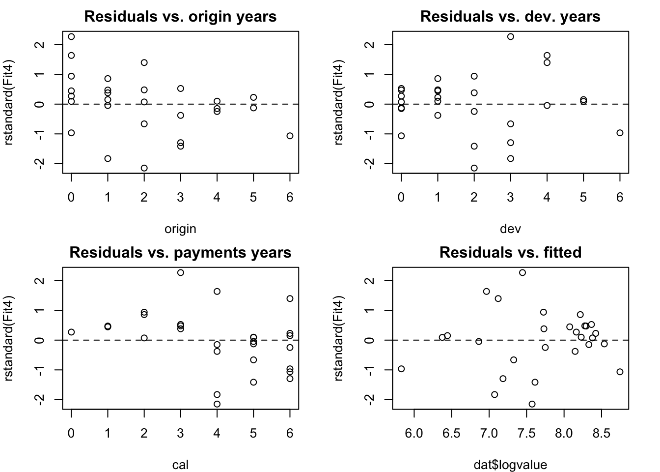

detach(model.frame(Fit4))
par(op)

op <- par(mfrow=c(2,2),oma = c(0, 0, 3, 0))
plot(Fit4)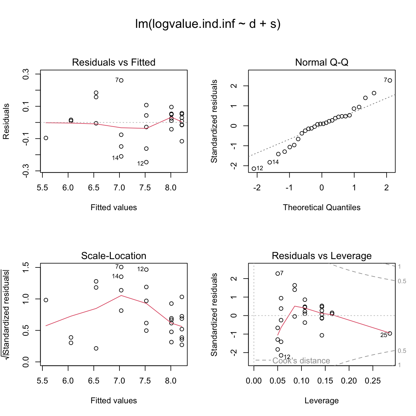

par(op)

I am happy with the model. To forecast the future claims payments I prepare a data frame with the predictors for those years.

# Tail of 6 more years over the observed period
tail.years <- 6
# Create a data frame for the future periods
fdat <- data.frame(
  origin = rep(0:(m-1), n+tail.years),
  dev = rep(0:(n+tail.years-1), each=m)
)

fdat <- within(fdat,{
  d <- ifelse(dev < 1, 1, 0)
  s <- ifelse(dev < 1, 0, dev)
  cal <- origin + dev
  a6 <- ifelse(origin == 6, 1, 0)
}) 

# New data
ND <- subset(fdat, cal>6)
ND <- merge(ND, ClaimsVolume)

Next I update my prediction function from last week with new parameters for claims inflation and indexation. The volume index and claims inflation parameters will be used to scale the output back to the original units and to inflated the future payments by a constant rate. Of course the indexation is a model in itself with uncertainty, which can be considered as part of the model error. Note, that I scale the data back to my volume index, but not earnings/inflation.

log.incr.predict <- function(
    model, # lm output
    newdata, # same argument as in predict
    claims.inflation=0, # Assumed inflation (scalar)
    volume.index=NULL, # name of the v.i. column in newdata  
    origin.var="origin", # name of the origin column in newdata
    dev.var="dev", # name of the dev column in newdata
    cal.var="cal" # name of the cal. period col. in newdata
){
  origin <- newdata[[origin.var]] 
  dev <- newdata[[dev.var]]
  cal <- newdata[[cal.var]]
  if(is.null(volume.index)){
    index <- 1
  }else{
    index <- newdata[[volume.index]]
  }
  Pred <- predict(model, newdata=newdata, se.fit=TRUE)
  
  Y <- Pred$fit
  VarY <- Pred$se.fit^2 + Pred$residual.scale^2 
  P <- exp(Y + VarY/2)
  P <- P*index*(1 + claims.inflation)^(cal - min(cal) + 1)
  VarP <-  P^2*(exp(VarY)-1)
  seP <- sqrt(VarP)
  
  ## Recreate formula to derive the model.frame and future design matrix   
  model.formula <- as.formula(paste("~", as.character(formula(model)[3])))
  ## See also package formula.tool
  
  mframe <- model.frame(model.formula, data=newdata)
  fdm <- model.matrix(model.formula, data=newdata)
  varcovar <- fdm %*% vcov(model) %*% t(fdm)
  
  sigma <- summary(model)$sigma
  dsigma2 = diag(sigma^2, nrow = dim(varcovar)[1])
  
  Total.SE <- sqrt( t(P) %*% (exp(dsigma2 + varcovar) - 1) %*% P )
  Total.Reserve <- sum(P)
  
  # Prepare output
  Incr=data.frame(origin, dev, Y, VarY, P, seP, CV=seP/P)
  out <- list(Forecast=Incr[order(newdata[[origin.var]]),],              
              Totals=data.frame(Total.Reserve, 
                                Total.SE=Total.SE, 
                                CV=Total.SE/Total.Reserve))
  return(out)
}

With my new prediction function it is easy to test different scenarios of claims inflations and their potential impact on the overall reserve requirements. Following the paper I will assume claims inflation of 7.5%. This gives me the following future payements triangle and reserves.

FM4 <- log.incr.predict(Fit4, ND,
                        claims.inflation=0.075, 
                        volume.index="volume.index")

# Page D5.41
round(xtabs(P ~ origin + dev, data=FM4$Forecast),0)

##       dev
## origin    1    2    3    4    5    6    7    8    9   10   11   12
##      0    0    0    0    0    0    0  249  165  109   72   47   31
##      1    0    0    0    0    0  412  272  179  118   78   52   34
##      2    0    0    0    0  703  464  306  202  134   88   58   39
##      3    0    0    0 1018  671  443  292  193  127   84   56   37
##      4    0    0 1585 1045  690  455  300  198  131   87   57   38
##      5    0 2945 1942 1280  845  557  368  243  160  106   70   46
##      6 6241 4114 2712 1788 1180  778  514  339  224  148   98   65

round(xtabs(seP ~ origin + dev, data=FM4$Forecast),0)

##       dev
## origin   1   2   3   4   5   6   7   8   9  10  11  12
##      0   0   0   0   0   0   0  36  25  18  13   9   6
##      1   0   0   0   0   0  55  39  27  19  14  10   7
##      2   0   0   0   0  90  62  44  31  22  16  11   8
##      3   0   0   0 125  86  59  42  29  21  15  11   7
##      4   0   0 192 129  88  61  43  30  21  15  11   8
##      5   0 358 235 158 108  75  52  37  26  19  13   9
##      6 777 500 329 220 151 105  73  52  37  26  19  13

FM4$Totals

##   Total.Reserve Total.SE         CV
## 1      38083.25 1724.987 0.04529515

Compared to the results of the previous week the overall reserves increased by £5,000, while the overall standard error has been reduced due to the smaller number of parameters. Chirstofides explains that the big increase in the overall reserves is largely driven by the most recent origin year, for which I have only one data point. From the residual plot I can see that the standardised residual for this point is about -1. This is not statistical significant, but I noticed that the highest value of the original triangle in development period 0 has become the lowest after the volume adjustments, see also the interaction plot at the top.

By putting the last origin period back into the model I get an output which is more in line with the result of last week.

# Page D5.42
log.incr.predict(lm(logvalue.ind.inf ~ a6 + d + s, dat), ND,
                 claims.inflation=0.075, 
                 volume.index="volume.index")$Totals

##   Total.Reserve Total.SE         CV
## 1      35901.59  2609.29 0.07267895

Conclusions

Reserving is always mixture of art and science, a combination of sound data analysis with expert judgement. A statistical data analysis can help to understand how much expert judgement is required. As Christofides points out in his closing remarks of section L, it is desirable to embed reserving into a Bayesian framework. Wayne Zhang has done some great research in this area. Yet, simple linear models are powerful tools to investigate the data. The model presented here can particularly help to investigate trends in the calendar/payement year direction. Those trend changes can highlight movements in claims inflation, or indeed changes in the claims settling process. Neither of those factors should be ignored.

The assumption that claims follow a log-normal distribution feels intuitively reasonable to me. Yet, the occasional negative incremental claim needs to be carefully considered. It certainly is a prompt to check if the assumption of log-normal distributed incremental claims is reasonable. Packages like car (Companion to Applied Regression) offer lots of diagnostic tools. Any pointers to how I could use those tools effectively will be much appreciated.

Barnett and Zehnwirth present a further idea to test these models by reducing the data for the fitting exercise and testing how stable the coefficients and predictions of the model are, see section 3.3 and table 3.3 in [2].

As usual the R code of this post is available as a gist on GitHub. The code on Github contains more details than presented here. It also includes examples from the Barnett and Zehnwirth paper mentioned above. Is there a demand to include the functions presented here into the ChainLadder package? Please get in touch.

References

[1] Stavros Christofides. Regression models based on log-incremental payments. Claims Reserving Manual. Volume 2 D5. September 1997

[2] Glen Barnett and Ben Zehnwirth. Best estimates for reserves. Proceedings of the CAS, LXXXVII(167), November 2000.

Session Info

R version 2.15.2 Patched (2013-01-01 r61512)
Platform: x86_64-apple-darwin9.8.0/x86_64 (64-bit)

locale:
[1] en_GB.UTF-8/en_GB.UTF-8/en_GB.UTF-8/C/en_GB.UTF-8/en_GB.UTF-8

attached base packages:
[1] stats     graphics  grDevices utils     datasets  methods   base     

loaded via a namespace (and not attached):
[1] tools_2.15.2