Now I see it! K-means cluster analysis in R

Of course, a picture on a computer monitor is a coloured plot of x and y coordinates or pixels. Still, I was smitten by David Sparks’ posts on is.r(), where he shows how easy it is to read images into R to analyse them. In two posts [1], [2] he replicates functionality of image manipulation programmes like GIMP.

I can’t resist to write about this here as well. David’s first post is about k-means cluster analysis. One of the popular algorithms for k-means is Lloyd’s algorithm. So, on that note I will use a picture of the Lloyd’s of London building to play around with David’s code, despite the fact that the two Lloyd have nothing to do with each other. Lloyd’s provides pictures of its building copyright free on its web site. However, I will use a reduced file size version, which I copied to GitHub.

The jpeg package by Simon Urbanek [3] allows me to load a jpeg-file into R. The R object of the images is an array, which has the structure of three layered matrices, representing the value of the colours red, green and blue for each x and y coordinate. I convert the array into a data frame, as this is an accepted structure by k-means and plot the data.

library(jpeg)
library(RCurl)
url <-"https://raw.githubusercontent.com/mages/diesunddas/master/Blog/LloydsBuilding.jpg"
readImage <- readJPEG(getURLContent(url, binary=TRUE))
dm <- dim(readImage)
rgbImage <- data.frame(
                    x=rep(1:dm[2], each=dm[1]),
                    y=rep(dm[1]:1, dm[2]),
                    r.value=as.vector(readImage[,,1]),
                    g.value=as.vector(readImage[,,2]),
                    b.value=as.vector(readImage[,,3]))

plot(y ~ x, data=rgbImage, main="Lloyd’s building",
     col = rgb(rgbImage[c("r.value", "g.value", "b.value")]), 
     asp = 1, pch = ".")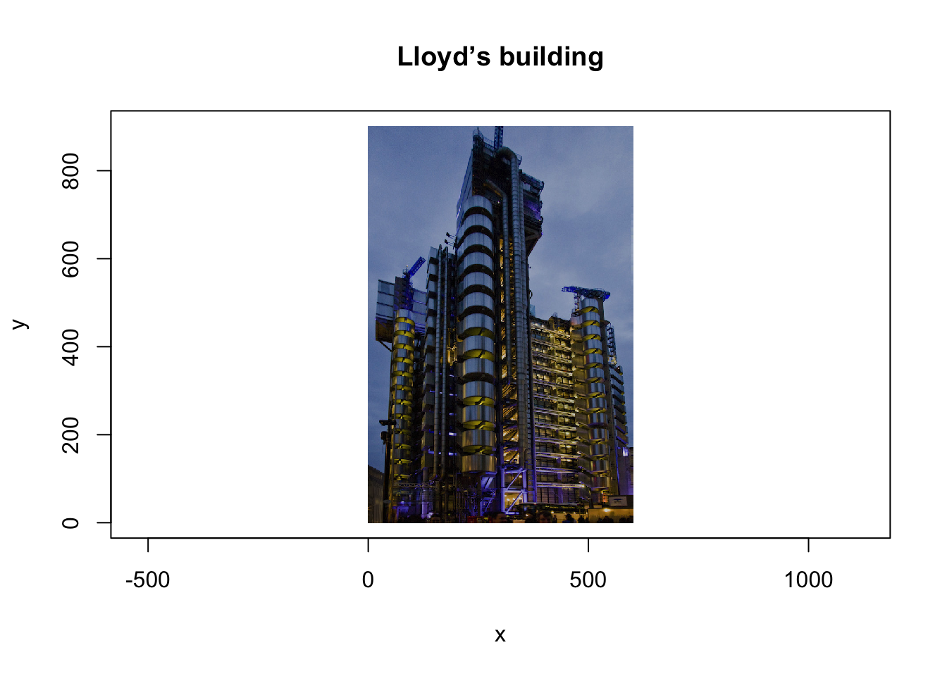

Running a k-means analysis on the three colour columns in my data frame allows me to reduce the picture to k colours. The output gives me for each x and y coordinate the colour cluster it belongs to. Thus, I plot my picture again, but replace the original colours with the cluster colours.

kColors <- 5  
kMeans <- kmeans(rgbImage[, c("r.value", "g.value", "b.value")], 
                 centers = kColors)
clusterColour <- rgb(kMeans$centers[kMeans$cluster, ])

plot(y ~ x, data=rgbImage, main="Lloyd’s building",
     col = clusterColour, asp = 1, pch = ".",
     axes=FALSE, ylab="", 
     xlab="k-means cluster analysis of 5 colours")

Running the k-means algorithm not only over the colours but over the whole data frame, including the x and y coordinate will find localised clusters, or so called Voronoi cells. This gives quite an artistic picture.

nRegions <- 2000 # Number of Voronoi cells. 
# Be patient, this takes time.
voronoiMeans <- kmeans(rgbImage, centers = nRegions, iter.max = 50)

## Warning: Quick-TRANSfer stage steps exceeded maximum (= 27000000)

voronoiColor <- rgb(voronoiMeans$centers[voronoiMeans$cluster, 3:5])

plot(y ~ x, data=rgbImage, col = voronoiColor, 
     asp = 1, pch = ".", main="Lloyd’s building",
     axes=FALSE, ylab="", xlab="2000 local clusters")

Instead of plotting all x and y coordinates I can also plot only the cluster centres. In the following chart I generated 500 cluster and plotted their centres as little rectangles, which provides an interesting picture in itself.

nRegions <- 500  
voronoiMeans <- kmeans(rgbImage, centers = nRegions, iter.max = 50)

## Warning: Quick-TRANSfer stage steps exceeded maximum (= 27000000)

voronoiColor <- voronoiColor <- rgb(voronoiMeans$centers[,3:5])

plot(y ~ x, data=voronoiMeans$centers, 
     col = voronoiColor, 
     main="Lloyd’s building", asp = 1, 
     pch = 15, cex=1.5, axes=FALSE, 
     ylab="", xlab="500 local clusters")

You can access the R-code of this post also as gist on Github. Many thanks again to David Sparks for his inspirations on is.R().

References

[1] David Sparks. Dominant color palettes with-k-means, is.R(). November 27, 2012
[2] David Sparks. Images as Voronoi tessellation, is.R(). November 28, 2012
[3] Simon Urbanek (2012). jpeg: Read and write JPEG images R package version 0.1.2.

Session Info

sessionInfo()

## R version 3.6.2 (2019-12-12)
## Platform: x86_64-apple-darwin15.6.0 (64-bit)
## Running under: macOS Catalina 10.15.3
## 
## Matrix products: default
## BLAS:   /Library/Frameworks/R.framework/Versions/3.6/Resources/lib/libRblas.0.dylib
## LAPACK: /Library/Frameworks/R.framework/Versions/3.6/Resources/lib/libRlapack.dylib
## 
## locale:
## [1] en_GB.UTF-8/en_GB.UTF-8/en_GB.UTF-8/C/en_GB.UTF-8/en_GB.UTF-8
## 
## attached base packages:
## [1] stats     graphics  grDevices utils     datasets  methods   base     
## 
## other attached packages:
## [1] RCurl_1.98-1.1 jpeg_0.1-8.1  
## 
## loaded via a namespace (and not attached):
##  [1] Rcpp_1.0.3      bookdown_0.17   digest_0.6.23   bitops_1.0-6   
##  [5] magrittr_1.5    evaluate_0.14   blogdown_0.17   rlang_0.4.4    
##  [9] stringi_1.4.5   rmarkdown_2.1   tools_3.6.2     stringr_1.4.0  
## [13] xfun_0.12       yaml_2.2.0      compiler_3.6.2  htmltools_0.4.0
## [17] knitr_1.27